
A video showing the Kollsman electric tachometer indicator ramping from 0% to 100% then 105%, 120%, back down to 100% then to 50%, 25%, and 5% then finally back down to 0%. At 100%, the three-phase, four-pole AC synchronous motor inside the indicator is spinning at 2100 RPM.
In this post, I take a look at a vintage Kollsman aircraft electric tachometer indicator. I start by disassembling the tachometer to determine how it works then build up a variable-frequency power supply to power and test the indicator. Once the power supply and indicator are working, I measure the speed of the motor inside the indicator to determine the number of poles on the motor. Finally, I repurpose this indicator as a unique CPU performance meter.
Outside Appearance
When I purchased the tachometer, I really had no idea what I was getting other than that it had an electrical interface rather than a mechanical flexible shaft interface and it looked cool.
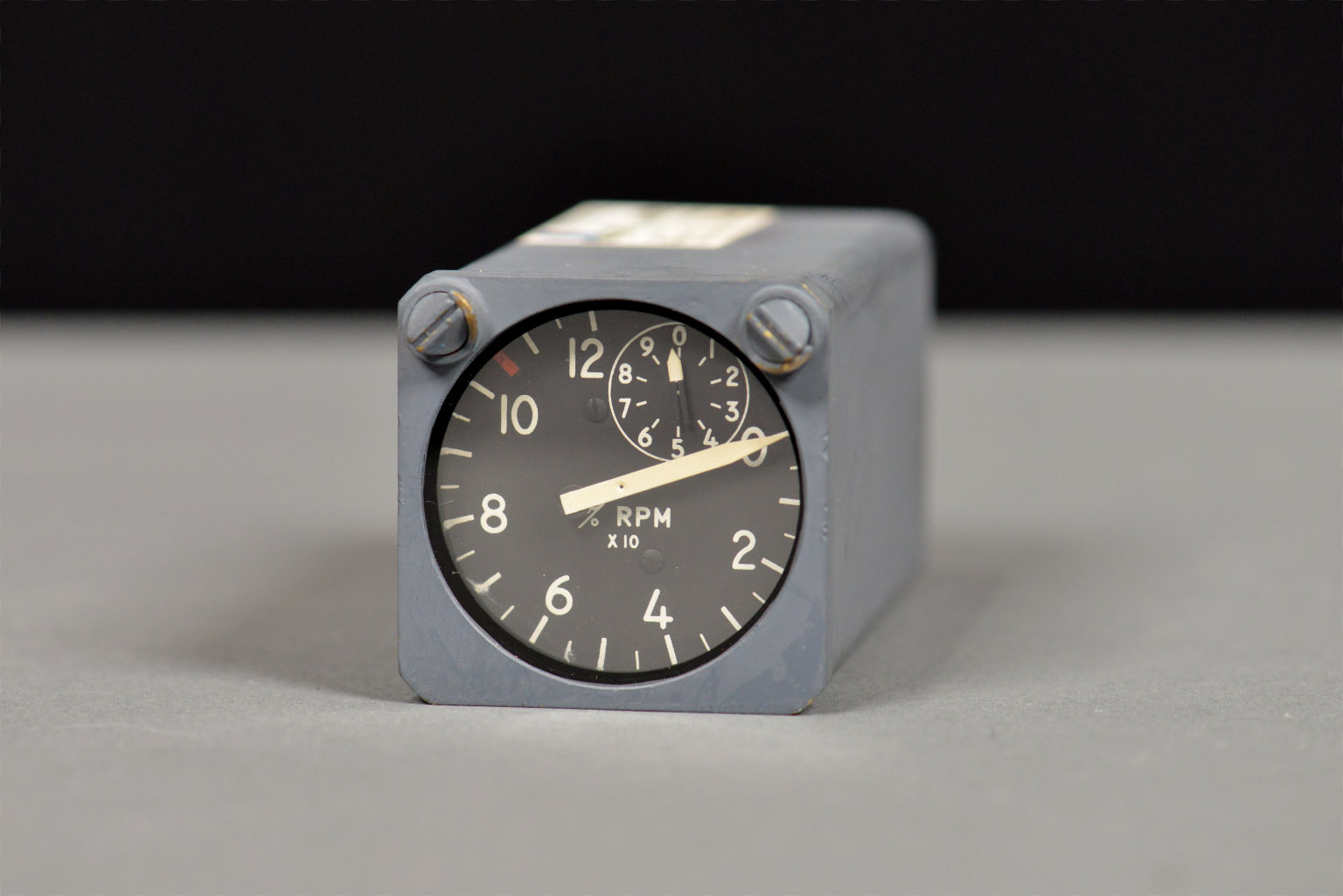
Front view of the Kollsman tachometer.
On the front of the unit are two dials. The larger dial indicates the tens digit of the percent of maximum RPM and the smaller inset dial indicates the ones digits. The two dials are added together to get the total percent. The larger dial red lines at 105% and goes all the way up to 120%.
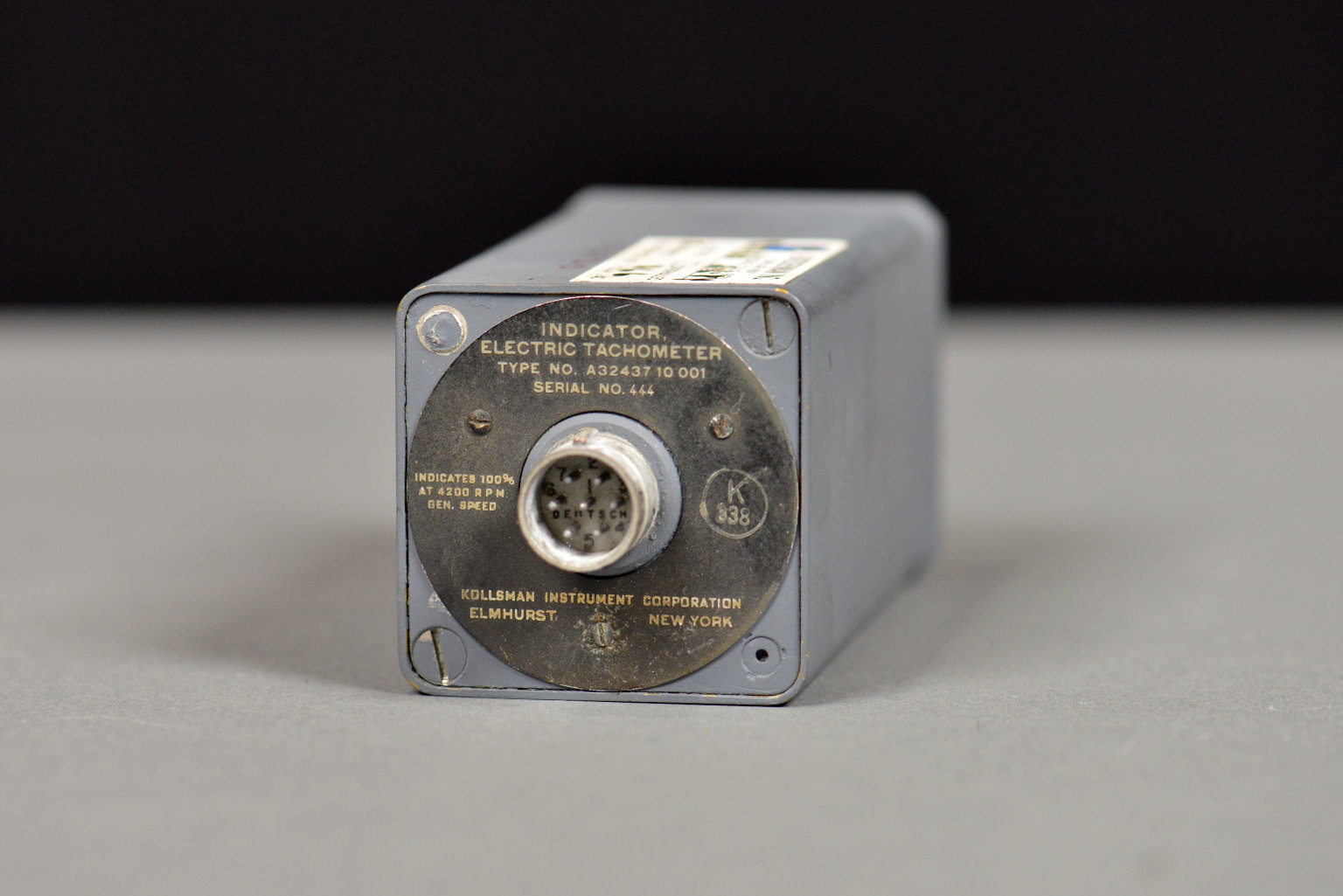
Rear view of the Kollsman tachometer.
On the rear is a receptacle with seven pin contacts and a nameplate. The nameplate lists the manufacturer, model number, serial number, and scale of the indicator. The scale is listed as “INDICATES 100% AT 4200 RPM GEN. SPEED.” The scale gives a little bit of information but still doesn’t convey how the speed of the engine is transmitted to the indicator. Maybe taking it apart would give me a better idea of how it works.
Disassembly
That wasn’t very helpful. The insides of the Kollsman tachometer.
Removing the two screws on the rear of the unit allowed the main body of the instrument to be slid out from its case. This did not reveal many secrets but it did allow for inspecting the dials and gears at the front of the indicator.

You can see the hairspring just behind the large main gear.
Pushing on the large needle showed that it was connected directly to the large gear immediately behind the face of the indicator via a small shaft. It also caused the small needle to spin very quickly. Releasing the needle caused both the large needle and small needle to spring back to zero. Looking closely there’s a hairspring behind the large gear near the face of the instrument. This hairspring is connected to the same shaft as the large gear and main needle and it’s this hairspring that causes the needles to spring back to zero when no force is applied to the shaft.
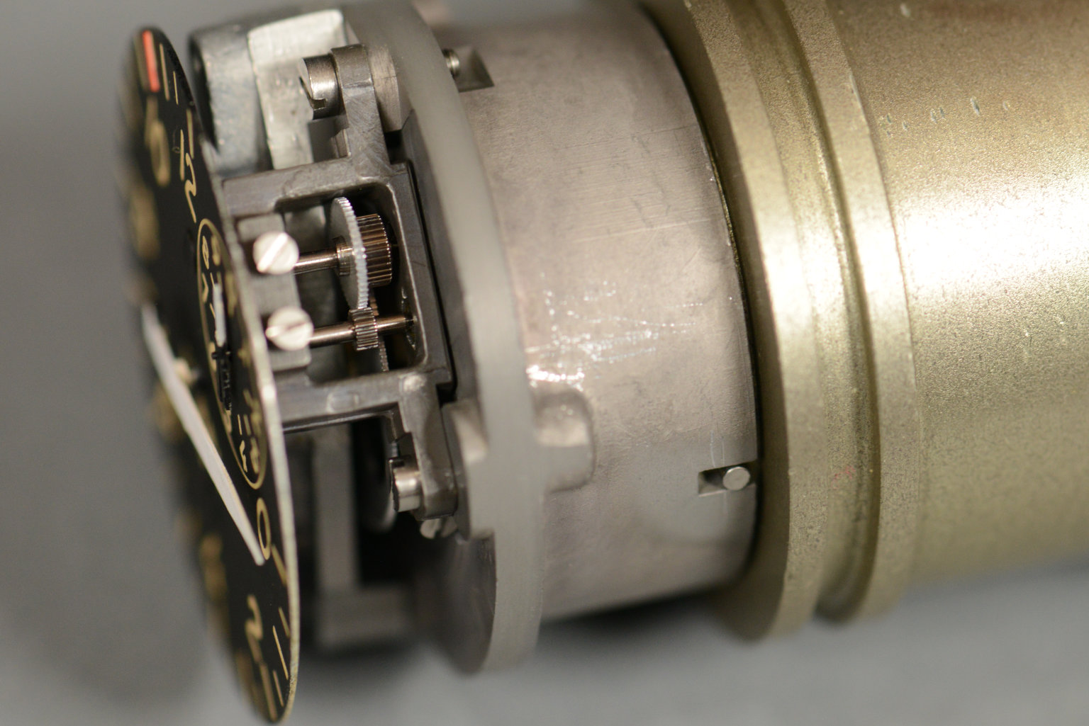
The large gear attached to the main dial’s needle turns a bunch of smaller gears connected to the small dial’s needle. This causes the small needle to spin very fast when the main needle changes quickly.
Looking at the right hand side of the front end of the indicator reveals that the large gear turns a bunch of smaller gears that are connected to the smaller needle. This causes the smaller needle to spin at a much faster rate than the main large needle.
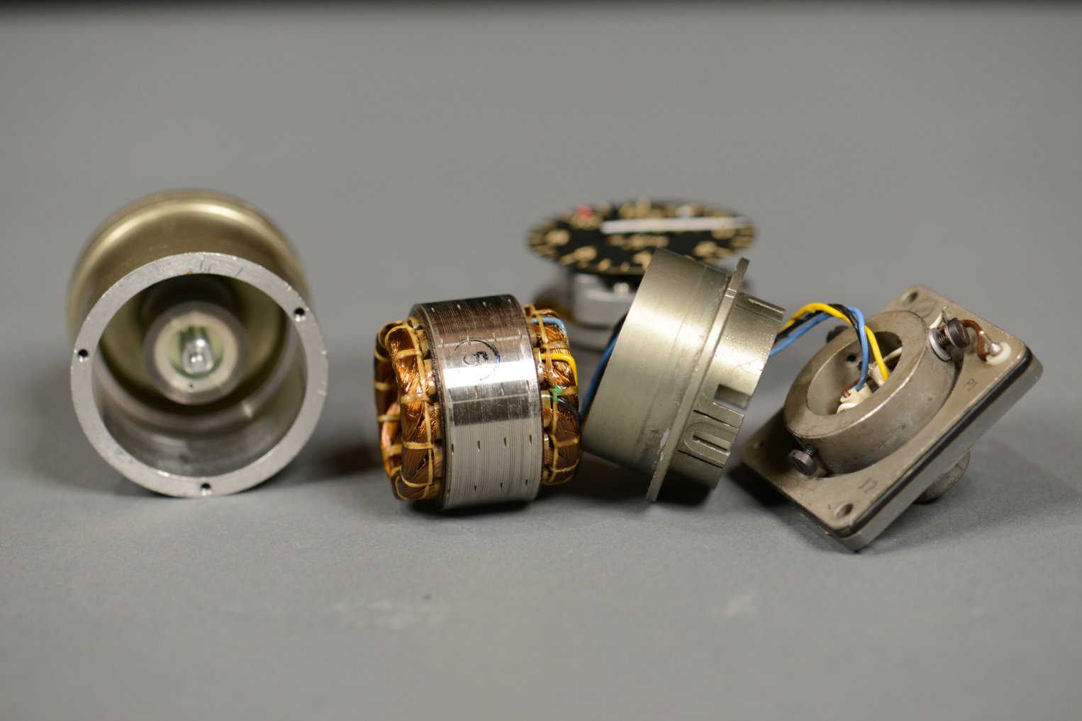
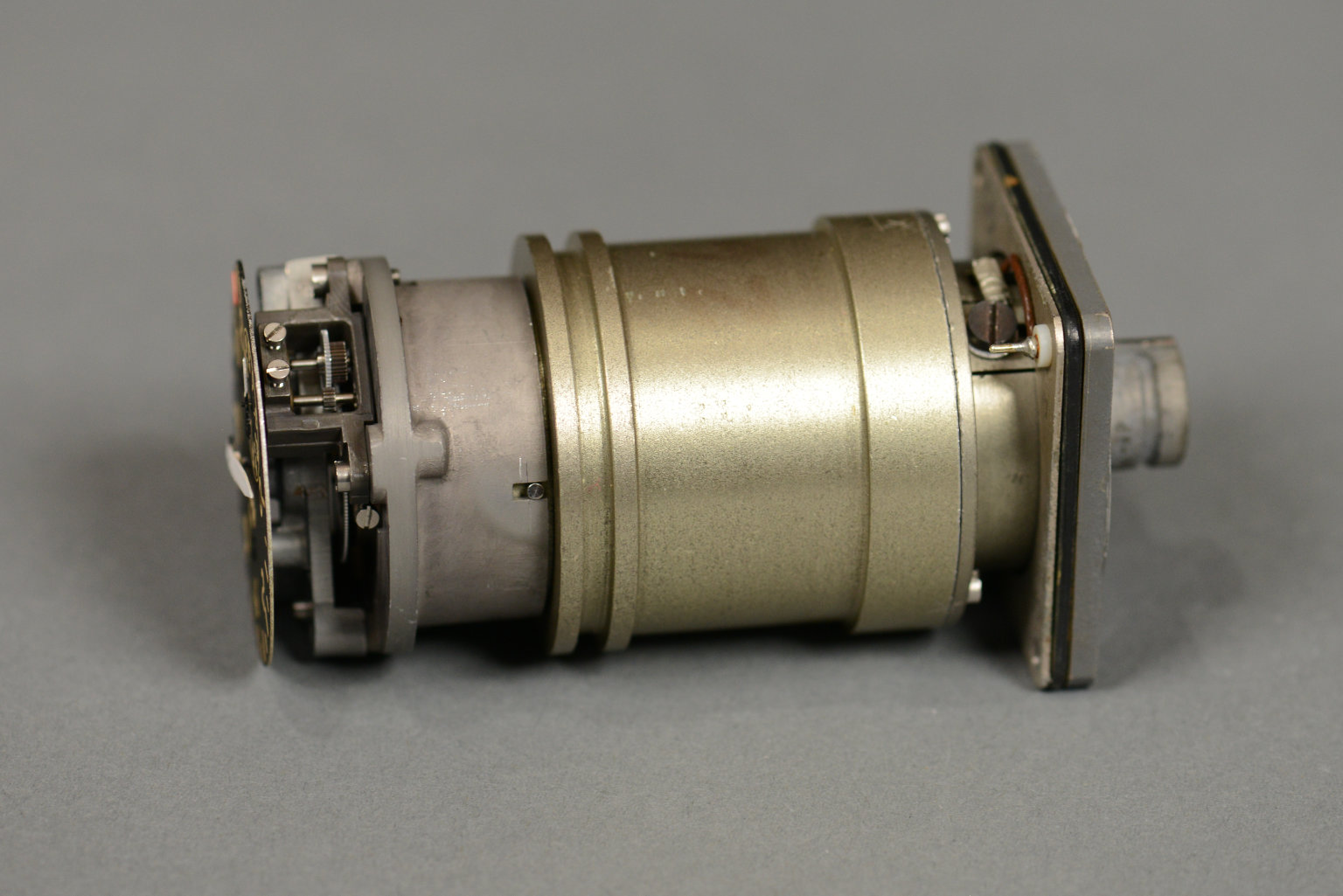
Opening up the main body reveals a three-phase synchronous motor. The tolerances between the stator and rotor are extremely tight. The rotor is the out of focus object inside the main body on the left. The stator consists of the metal ring and copper windings in the center.
The next step was to separate the main body from the rear panel and indicator dials then disassemble the main body. Removing the rear panel from the main body revealed yellow, black, and blue wires going into the body and two wires used for illumination. Removing the rear panel also allowed access to three small screws that when removed permitted the main body to be disassembled.
Disassembling the main body showed it housed a three-phase synchronous motor. The rotor spins on bearings located at the front and rear of the main body and fits inside the stator. The yellow, black, and blue wires are connected directly to the stator windings. The stator windings look to be divided into 12 groups so this is likely a four-pole motor. There are no brushes in the motor or windings on the rotor.
The clearances between the rotor and stator are very tight. It took several tries to get the main body reassembled where the rotor would spin freely inside the stator but I did eventually get it back together and working again.
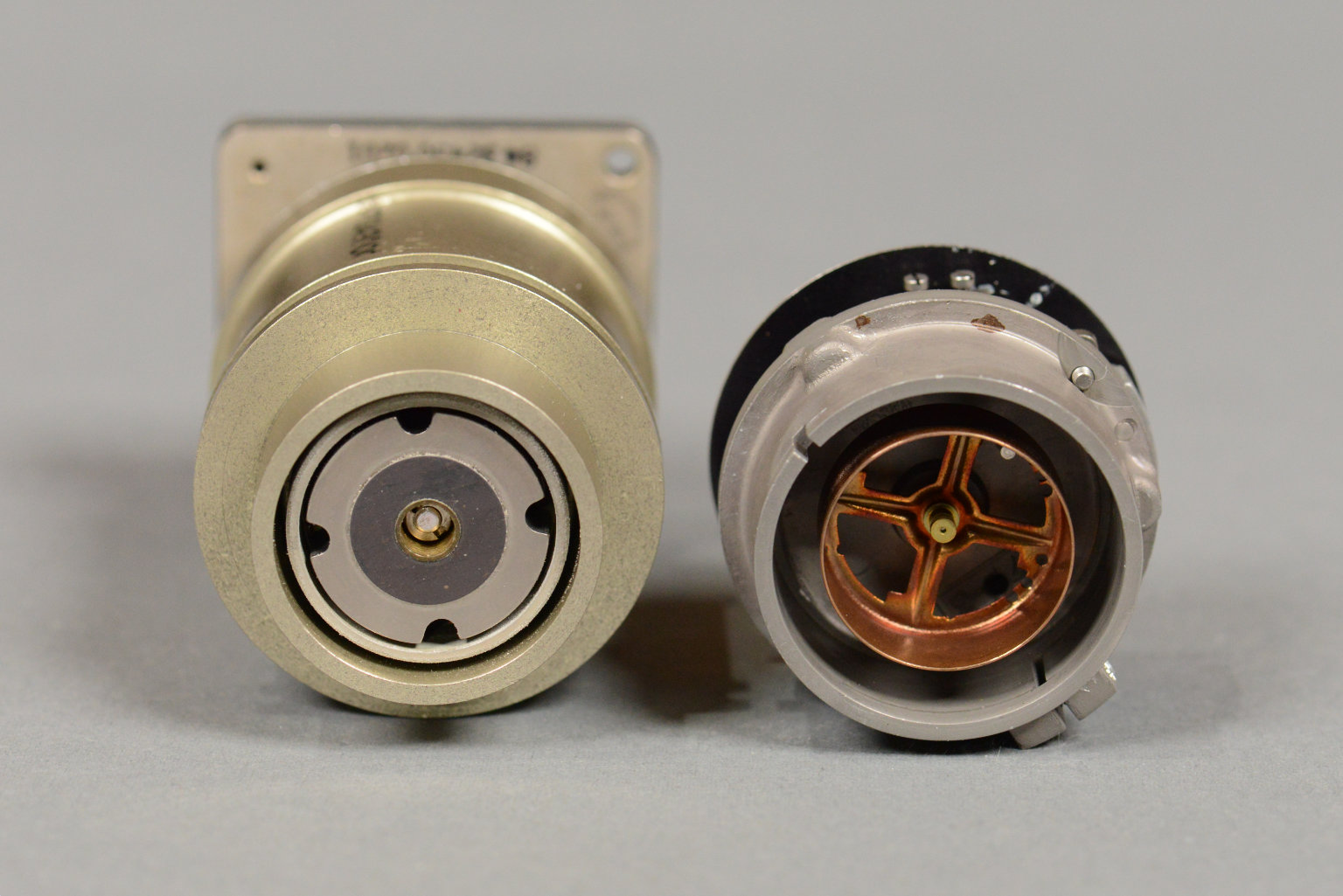
Removing the indicator from the main body reveals the magic…a rotating magnet and iron shield on the motor side and a copper cup on the dial and needle side.
The magic happens at the end of the main body near the front face of the indicator. On this end of the main body are a large round magnet that spins and is attached to the rotor. Around the magnet is an iron shield that spins with the magnet.
On the indicator side is a copper cup. The copper cup fits into the gap between the magnet and shield but does not make physical contact with the magnet or shield. The copper cup is connected to the same shaft that is connected to the hairspring, large gear, and large needle on the front of the unit.
Since the magnet and shield spin but do not make contact with the copper cup and copper is a nonferrous metal, some mechanism is needed to turn the spinning of the magnet into a force on the cup to turn the shaft to turn the needles. Time to do some research!
Magnetic Drag Cup Tachometers
After doing a bit of looking around, I learned that this is called a magnetic drag cup tachometer. The rotating magnet induces Eddy currents in the copper cup which causes the copper cup to rotate and apply a force to the shaft that counteracts the force applied by the hairspring. The shaft rotates and the pointer moves to the point where the balance of the two forces is equal. The faster the magnet spins, the greater the currents induced in the copper cup, the greater the force produced on the shaft to counteract the hairspring, and the greater the deflection of the pointer away from 0%.
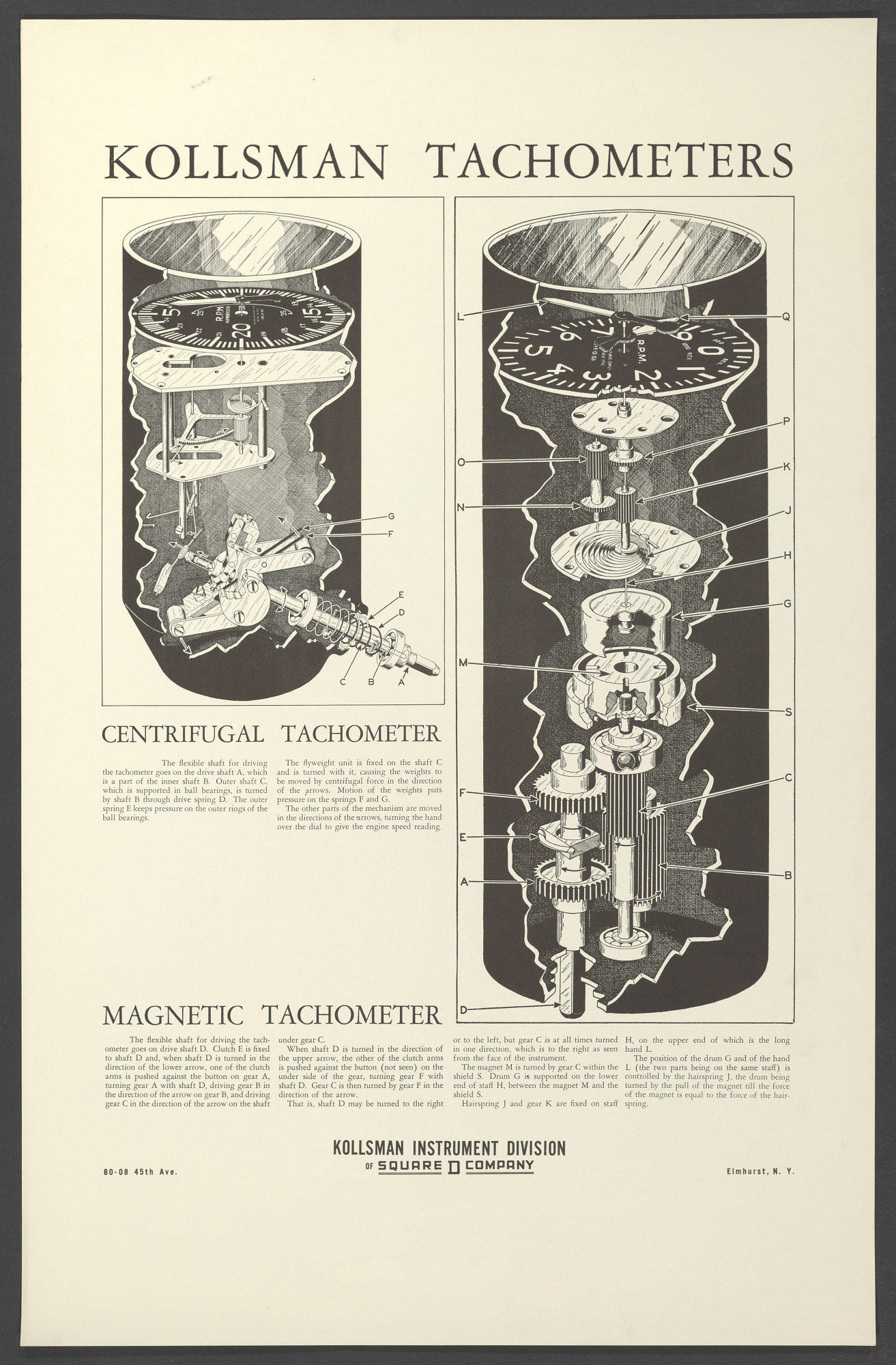
Kollsman Tachometers poster from the Smithsonian Institution.
The best illustration of the magnetic drag cup tachometer is on the Kollsman poster shown above from the Smithsonian Institution’s National Air and Space Museum collection. This poster depicts a magnetic drag cup tachometer connected to the engine through the use of a flexible rotating shaft. The explanation reads:
The flexible shaft for driving the tachometer goes on drive shaft D. Clutch E is fixed to shaft D and, when shaft D is turned in the direction of the lower arrow, one of the clutch arms is pushed against the button on gear A, turning gear A with shaft D, driving gear B in the direction of the arrow on gear B, and driving gear C in the direction of the arrow on the shaft under gear C.
When shaft D is turned in the direction of the upper arrow, the other of the clutch arms is pushed against the button (not seen) on the under side of the gear, turning gear F with shaft D. Gear C is then turned by gear F in the direction of the arrow.
That is, shaft D may be turned to the right or to the left, but gear C is at all times turned in one direction, which is to the right as seen from the face of the instrument.
The magnet M is turned by gear C within the shield S. Drum G is supported on the lower end of staff H, between the magnet M and the shield S.
Hairspring J and gear K are fixed on staff H, on the upper end of which is the long hand L.
The position of the drum G and of the hand L (the two parts being on the same staff) is controlled by the hairspring J, the drum being turned by the pull of the magnet till the force of the magnet is equal to the force of the hairspring.
The core functioning of the magnetic tachometer on this poster is identical to my tachometer. The main difference is that my tachometer has a synchronous AC motor that turns shaft C instead of a flexible rotating shaft. The other major difference is that the face of my tachometer has two dials to represent the tens and units rather than a pair of concentric pointers.
Electrical Coupling Using AC Synchronous Machines
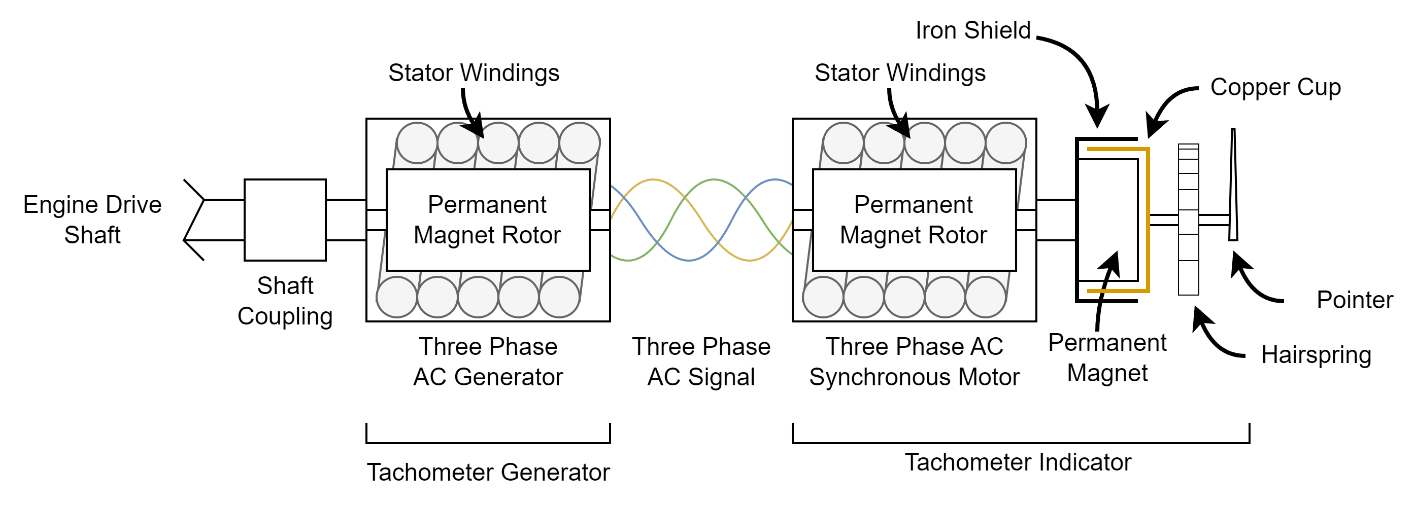
Tachometer generator – tachometer indicator system.
In the drag cup tachometer on the Kollsman poster, the speed of the engine is conveyed from the engine to the tachometer by means of a flexible rotating shaft. In my tachometer, the speed of the engine is conveyed from the engine to the tachometer by means of a three-phase AC generator, a three-phase AC signal transmitted over three electrical conductors, and a three-phase synchronous AC motor as shown in the diagram above.
The engine drive shaft is coupled to a three-phase AC generator. The generator produces a three-phase AC output whose frequency is proportional to the rotational speed of the engine drive shaft. In the case of a two-pole AC generator spinning at 4200 RPM, the output frequency will be 70 Hz. If the same generator is spinning at half that speed, the frequency will be halved to 35 Hz. If the generator is stopped, no voltage will be output.
Wires connect the tachometer generator to the tachometer indicator. Inside the tachometer indicator, the three-phase AC signal from the generator turns a three-phase AC synchronous motor. The speed of the motor will be proportional to and synchronous to the input frequency. If the synchronous motor also has two poles, the motor will spin at the exact same speed as the two-pole generator.
In other words, a 4200 RPM drive shaft will produce a 70 Hz signal at the output of a two-pole generator and a 70 Hz signal at the input to a two-pole motor will cause the motor’s shaft to rotate at 4200 RPM. If the drive shaft is slowed to 2100 RPM, the generator output is reduced to 35 Hz and the motor’s shaft’s speed will also be reduced to 2100 RPM. In this way, the speed of the drive shaft is conveyed from the engine to the tachometer indicator.
The motor’s shaft spins a permanent magnet drum and iron shield. A copper cup is placed around the drum. As the drum rotates, it induces Eddy currents in the copper cup. The copper cup becomes magnetic and exerts a force on the shaft connecting it to the hairspring and indicator pointer. The higher the speed of the drum, the greater the induced currents and the greater the force applied to the pointer’s shaft.
The needle will then move to the point where the force applied by the copper cup is equal to the counteracting force applied by the hairspring. This causes the pointer to move over an angle in proportion to the frequency of the AC signal at the input of the tachometer indicator which is also proportional to the speed of the engine drive shaft at the tachometer generator.
Another explanation of this system is on pages 4 to 7 of chapter 6 of the Small Gas Turbine Engines Handbook by Ian F Bennett at gasturbineworld.co.uk. Ian also notes that many of these gauges indicate 100% when driven by a 4200 RPM two-pole generator which corresponds to a 70 Hz AC signal. Hmm, that’s exactly the scale mentioned on the nameplate on my tachometer.
The 3-Phase Variable-Frequency AC Power Supply
Power Supply Requirements
After disassembling this indicator, putting it back together, and researching how it works, I decided it was time to get it running again! I don’t have a jet engine or tachometer generator so I figured the next best thing was to build a three-phase AC power supply. I came up with the following list of requirements:
- Continuously variable frequency from DC to 120% of 70 Hz (84 Hz).
- An adjustable voltage output. I have no idea what voltage the motor is designed to run from.
- Able to supply a few 10’s of mA of current per phase. I have no idea how much current the motor pulls.
Fortunately, I already had a small board capable of generating a three-phase AC signal. The voltage is adjustable from 0 to 7.25 VAC and it is capable of supplying a few 10’s of mA of current per phase. This board would be enough to try to figure out the unknowns in the list of requirements above.
Power Supply Schematic

Three-phase AC power supply schematic.
This is a three-phase version of the single-phase AC power supply used on my synchro-to-digital converter project. The number of channels has been increased from one to three and the Pimoroni Tiny 2040 has been replaced by a seven pin header that connects to an off-board Raspberry Pi Pico RP2040 development board. Each DAC has its own SPI chip select signal so that they may be operated independently. Please see the Constructing a Reference Voltage Source section of that post for the theory of operation behind the power supply.
Power Supply Board Design
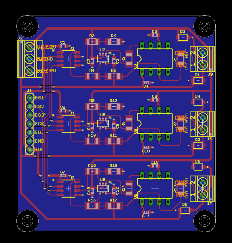
Three-phase AC power supply board design.
The power supply board layout is shown above. It is the same layout duplicated three times. A ±12 volt power supply connects in the upper left. Centered on the left edge is the 7 pin header that connects to the RP2040 Pico development board. On the right edge are the three output channels. Phase 1 is at the top, phase 2 is in the middle, and phase 3 is at the bottom. These are controlled by the DACs connected to /CS1, /CS2, and /CS3 respectively.
Board Assembly
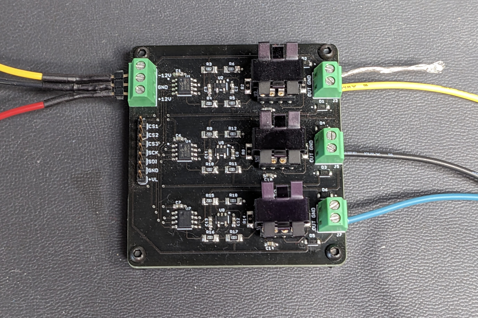
The complete power supply board. It’s been on the bench for a while so it’s gotten quite dusty. The bare ground lead is for connecting scope probe grounds.
The assembled board is shown above. The LT1010 buffers have small heatsinks to help with heat dissipation. I was out of right-angle headers at the time so I used a straight header for the connections to the Pico development board.
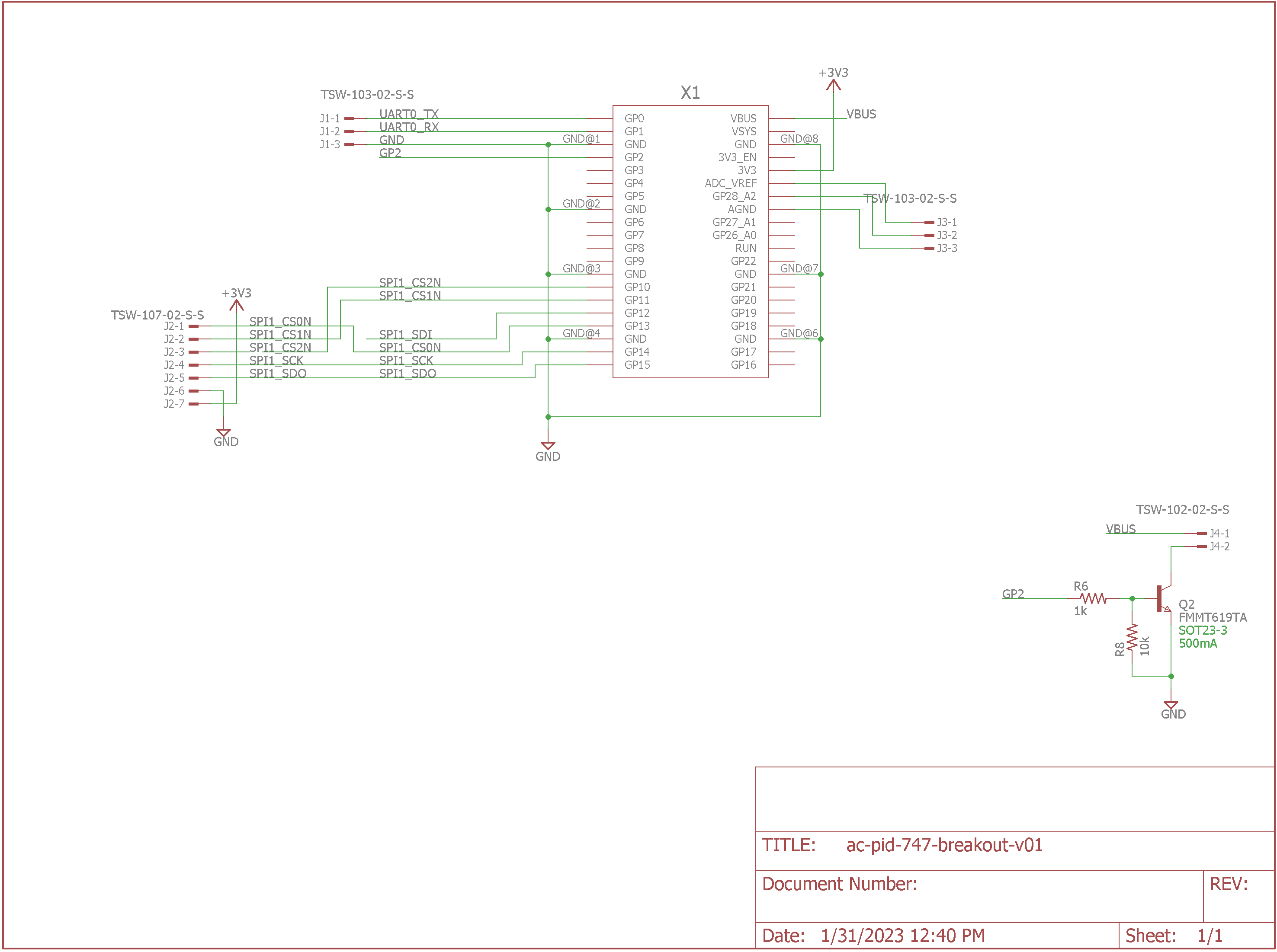
Schematic of the breakout board used to connect the Pico development board to the power supply board.
Instead of having a bunch of jumper wires running between the power supply board and the Pico development board, I built another small board to route the SPI connections from the Pico to the power supply board. It also breaks out a serial port and provides some connections to some hardware used on a different project.

The power supply board with the Raspberry Pi Pico development board attached.
A photo of my two boards and the Pico development board connected together is shown above. This is the point at which I wish I would have waited and used a right-angle header on the power supply board. But, hey, it works.
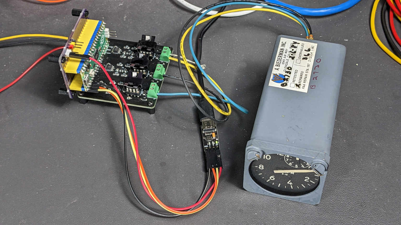
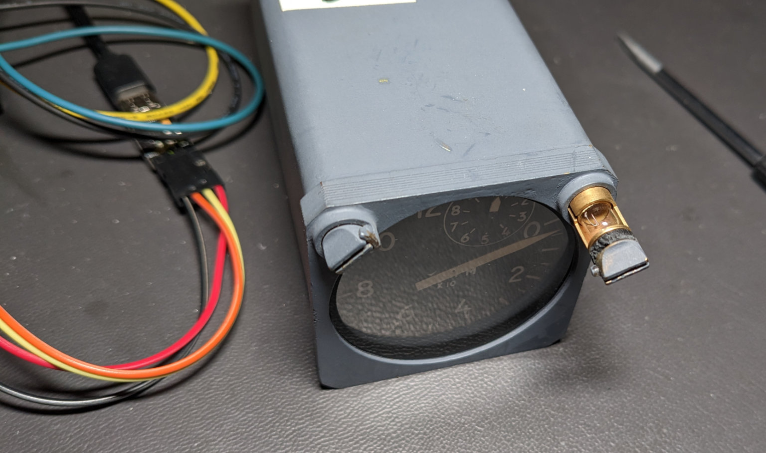
The complete test setup including the tachometer.
The photo above shows the complete test setup. The small board is an FTDI USB to UART board to power and communicate with the Pico development board.
Direct Digital Synthesis
This project uses direct digital synthesis to generate three sine waves with a programmable frequency that are separated by 120°. The basics of direct digital synthesis are covered very well by articles on the Analog Devices, Digi-Key, and DSP Related websites among others. V. Hunter Adams has a great explanation with animations and example Python code and even an RP2040 implementation on his website. Rather than get into the fundamentals of DDS in this blog post, I’ll cover just the details specific to this implementation.
I selected the following parameters for my frequency synthesizer:
| Parameter | Value |
|---|---|
| Sampling Frequency | 10 kHz |
| Tuning Word Size | 32 bits, unsigned |
| Phase Accumulator Size | 32 bits, unsigned |
| Scale Size | single-precision float |
| Number of Outputs | 3 outputs separated by 120° |
With a 10 kHz sampling frequency, the DDS NCO could produce a frequency anywhere from to DC to 5 kHz with an appropriate analog low pass filter after the DAC. My actual maximum frequency in practice will be 120% of 70 Hz or 84 Hz. I don’t have a low-pass filter on my power supply board but since I’m massively oversampled (fmax of 84 Hz vs fs of 10 kHz), it will be fine.
I selected a word size of 32 bits for both the tuning word and phase accumulator register since that’s the native size of an unsigned integer on the RP2040 microcontroller. I decided to use a single-precision float for the scale. The RP2040 microcontroller has plenty of power to perform 3 floating point multiplies per sample period and using floats was easier than figuring out the fixed-point math to perform similar scaling using integers.
The final complication is that I need to produce three outputs at the same frequency but separated by 120°. I came up with the following block diagram for my three-phase synthesizer. The logic in this block diagram is executed once per sample period (10,000 times per second):
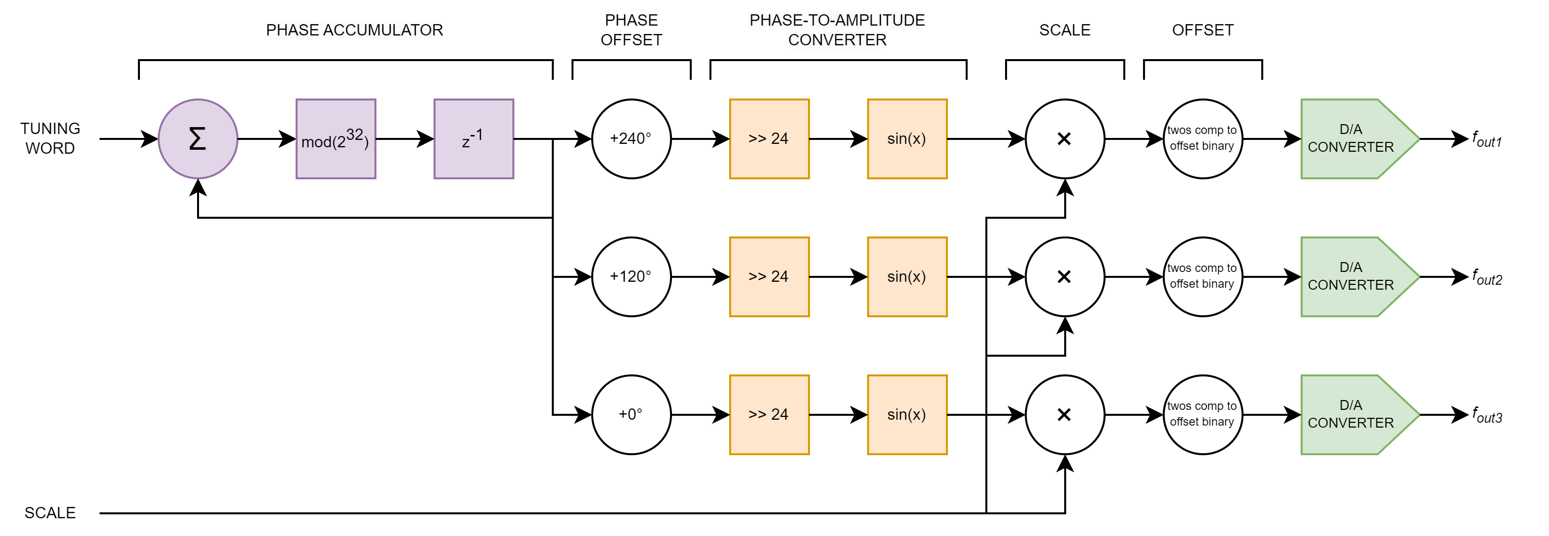
Three-phase frequency synthesizer as used in this project.
On the left are the inputs to the logic. These include the tuning word for adjusting the frequency and the scale value for adjusting the final output level. The phase accumulator is shown in purple above. The tuning word is added to the last value of the accumulator, wrapped modulo 232, then saved for the next run of the code.
240°, 120°, and 0° are added to the output of the phase accumulator to produce three signals offset 120° from each other. A phase offset of 240° corresponds to adding modulo 232 a value of 2/3 × 232 = 2863311531 to the output of the phase accumulator and a phase offset of 120° corresponds to adding modulo 232 a value of 1/3 × 232 = 1431655765 to the output of the phase accumulator.
The phase-to-amplitude converters are shown in orange above. My sine lookup table only has 256 entries of 8 bits each therefore, I’m only using the upper 8 bits of the phase accumulator to produce the sin(x) output. Dropping the lower 24 bits of the 32 bit phase values gets an 8 bit value that used as an index into the sine lookup table.
The three sine values are then multiplied by the scale and converted from two’s complement value to offset binary values for the DACs. Finally the offset binary sine waves are sent to the DACs using a SPI interface.
The value of the tuning word in terms of the output frequency, fo, phase accumulator width in bits, N, and sampling frequency, fs, is given by the following formula:
$$ tuning\ word = \frac{f_o\ ×\ 2^N}{f_s}$$
In our system, fo ranges from 0 to 84 Hz, N is 32, and fo is 10 kHz. Let’s calculate some useful tuning words for our tachometer:
| Percent Max RPM | fo | Tuning Word |
|---|---|---|
| 120% | 84.0 Hz | 36077725 |
| 105% | 73.5 Hz | 31568010 |
| 100% | 70.0 Hz | 30064771 |
| 75% | 52.5 Hz | 22548578 |
| 50% | 35.0 Hz | 15032386 |
| 25% | 17.5 Hz | 7516193 |
| 0% | 0 Hz | 0 |
If you know the value of the tuning word, you can determine the output frequency given the following formula:
$$f_o = \frac{tuning\ word\ ×\ 2^N}{f_s}$$
Software
The software for this project is divided into two main parts. The first part runs on core 0, accepts a percent value from the user to display on the indicator, and then ramps the percent displayed on the indicator from the current value to the user’s entered value over time. The second part runs on core 1, performs direct digital synthesis of the three-phase signal, and writes the waveform to the DACs.
The User Input Thread on Core 0
The user input thread runs inside the main loop on core 0. It consists of fast tasks that execute as often as they can and slow tasks that run 100 times per second. The pacing of the slow tasks is performed using a flag that is set inside a repeating timer function that runs at 100 Hz on the default thread pool on core 0. When the main loop code sees the flag is set, it clears the flag then runs the 100 Hz tasks.
Let’s start with the fast tasks:
    // main loop
    while (1) {

        //----------------------------------------
        // fast tasks
        //----------------------------------------
I have a command line editor that I’ve been using for decades now. The GetCommand function checks the Pico’s serial port for a new character then appends the character to the current command line or takes action to perform deletes, rub outs, or carriage returns.
        // run get command state machine to get a line of input (non-blocking)
        GetCommand ();
When a complete command line is available, the command line editor sets the value of cmd_state to 2. This is the main loop’s signal that it’s time to process the command line in the cmd_buffer. The following code detects this then starts splitting out the arguments which are separated by a comma:
        // once a line of input is received, process it
        if (cmd_state == 2) {
            int index = 0;
            char *buffptr = strtok (cmd_buffer, ",");
            while (buffptr != NULL) {

                switch (index++) {
The following code takes a percentage entered on the command line and converts it into the target tuning word for the frequency synthesizer:
                    case 0:
                        newPercent = atof (buffptr);
                        newAdderTarget = newPercent / 100.0 * 30064771.0;
                        printf ("newAdderTarget: %ld\n", newAdderTarget);
                        break;
The following code processes any remaining arguments then sets the cmd_state to 0. The is the command line editor’s signal to reset the command line editor and start to accept a new line of text:
                    default:
                        printf ("detected an unused argument\n");
                        break;
                }
                buffptr = strtok (NULL, ",");
            }
            cmd_state = 0;
        }
After processing the command line arguments, the main loop checks to see if it’s time to execute the 100 Hz tasks:
        //----------------------------------------
        // 100 Hz tasks
        //----------------------------------------

        if (flag100) {
If it is, it clears the flag then runs the 100 Hz tasks:
flag100 = false;
Like blinking the LED in a fancy pattern:
            // blink led
            if (ledTimer == 0) {
                // led on
                gpio_put (LED_PIN, 1);
            } else if (ledTimer == 25) {
                // led off
                gpio_put (LED_PIN, 0);
            }

            // increment led timer counter, 1 second period
            if (++ledTimer >= 100) {
                ledTimer = 0;
            }
And ramping the tuning word from its current value to the target value set from the command line. The slow ramp is performed to simulate how a tachometer generator connected to a real engine might ramp or down in RPMs. The tachometer indicator will stutter some or even stop tracking the RPMs if the frequency is changed abruptly:
            if (newAdderTarget > newAdder) {
                if ((newAdderTarget - newAdder) < rate) {
                    newAdder = newAdderTarget;
                } else {
                    newAdder += rate;
                }
                // printf ("(+) %d\n", newAdder);
            } else if (newAdderTarget < newAdder) {
                if ((newAdder - newAdderTarget) < rate) {
                    newAdder = newAdderTarget;
                } else {
                    newAdder -= rate;
                }
                // printf ("(-) %d\n", newAdder);
            }
An AC generator’s voltage is proportional to its speed so I ramp the voltage up and down with the frequency. The voltage ramping is subject to limits of 0.2 to 0.5 of full scale and is set to 0 at 0 Hz:
            // compute scale from frequency control word
            newScale = (float)newAdder * 0.50 / 36077725.2 + 0.2;
            if (newScale > 0.5) {
                newScale = 0.5;
            }
            if (newAdder == 0) {
                newScale = 0;
            }
The last step is to communicate the current tuning word and scale values to the direct digital synthesis thread running on core 1 using a critical section and a few global variables:
            // update speed and direction for core 1 ISR
            critical_section_enter_blocking (&scale_critsec);
            sin_adder = newAdder;
            scale = newScale;
            critical_section_exit (&scale_critsec);
        }
The end of the main loop:
}
Communicating Between Cores
My code uses a critical section to communicate the phase adder and gain between the UI thread running on core 0 and the DDS thread running on core 1. If one thread is already executing the code in a critical section, the second thread will wait until the first thread is done executing the code in the critical section before it starts executing it.
To use a critical section, we need to declare it plus some global variables that will be shared by the two threads:
critical_section_t scale_critsec;
static volatile uint32_t sin_adder = 0;
static volatile float scale = 0.0;
The critical section must be initialized before use. I did this just inside the main function before starting the second core:
    // initialize critical section
    critical_section_init (&scale_critsec);
When the first thread wants to write these globals, it enters the critical sections, performs the writes, then exits the critical section. This code in the UI thread writes the new phase adder and new scale to the global variables used to communicate with the DDS thread:
   // update phase adder and scale for core 1 ISR
   critical_section_enter_blocking (&scale_critsec);
   sin_adder = newAdder;
   scale = newScale;
   critical_section_exit (&scale_critsec);
When the second thread wants to read these globals, it enters the critical sections, performs the writes, then exits the critical section. This code adds the phase adder to the phase accumulator then makes a local copy of the gain to apply to the output waveforms:
    critical_section_enter_blocking (&scale_critsec);
    sin_phase += sin_adder;
    localScale = scale;
    critical_section_exit
The Direct Digital Synthesis Thread on Core 1
Let’s walk through the direct digital synthesis code. We’re generating sine waves so we need to compute the value of sin(x) quickly. A table lookup is likely faster than using the Pico’s floating point math library. Even though I stuffed the board with the 12-bit MCP4822 DAC, I’m only using 8 of those bits so a table with 256 8-bit values is sufficient:
// sine lookup table
// round(sin((0:255)*2*pi/256)*127);
static const int8_t sine[256] = {
     0,    3,    6,    9,   12,   16,   19,   22,   25,   28,   31,   34,   37,   40,   43,
    46,   49,   51,   54,   57,   60,   63,   65,   68,   71,   73,   76,   78,   81,   83,
    85,   88,   90,   92,   94,   96,   98,  100,  102,  104,  106,  107,  109,  111,  112,
   113,  115,  116,  117,  118,  120,  121,  122,  122,  123,  124,  125,  125,  126,  126,
   126,  127,  127,  127,  127,  127,  127,  127,  126,  126,  126,  125,  125,  124,  123,
   122,  122,  121,  120,  118,  117,  116,  115,  113,  112,  111,  109,  107,  106,  104,
   102,  100,   98,   96,   94,   92,   90,   88,   85,   83,   81,   78,   76,   73,   71,
    68,   65,   63,   60,   57,   54,   51,   49,   46,   43,   40,   37,   34,   31,   28,
    25,   22,   19,   16,   12,    9,    6,    3,    0,   -3,   -6,   -9,  -12,  -16,  -19,
   -22,  -25,  -28,  -31,  -34,  -37,  -40,  -43,  -46,  -49,  -51,  -54,  -57,  -60,  -63,
   -65,  -68,  -71,  -73,  -76,  -78,  -81,  -83,  -85,  -88,  -90,  -92,  -94,  -96,  -98,
  -100, -102, -104, -106, -107, -109, -111, -112, -113, -115, -116, -117, -118, -120, -121,
  -122, -122, -123, -124, -125, -125, -126, -126, -126, -127, -127, -127, -127, -127, -127,
  -127, -126, -126, -126, -125, -125, -124, -123, -122, -122, -121, -120, -118, -117, -116,
  -115, -113, -112, -111, -109, -107, -106, -104, -102, -100,  -98,  -96,  -94,  -92,  -90,
   -88,  -85,  -83,  -81,  -78,  -76,  -73,  -71,  -68,  -65,  -63,  -60,  -57,  -54,  -51,
   -49,  -46,  -43,  -40,  -37,  -34,  -31,  -28,  -25,  -22,  -19,  -16,  -12,   -9,   -6,
    -3
};
The core1_entry function is the start of the thread running on core 1. It creates a new alarm pool running on the core then starts a repeating timer that runs every 100 µs (10 kHz). Once the timer is created, this function has nothing else to do so it busy waits:
void core1_entry (void)
{
    // local system variables
    alarm_pool_t *core1_alarm_pool;
    struct repeating_timer timer_10kHz;

    // create new alarm pool
    core1_alarm_pool = alarm_pool_create (2, 16);

    // run 10 kHz timer interrupt on core 1
    alarm_pool_add_repeating_timer_us (core1_alarm_pool,
        -100, repeating_timer_callback_10kHz, NULL, &timer_10kHz);

    // nothing else to do on core 1
    while (1) {
        tight_loop_contents ();
    }
}
The repeating_timer_callback_10kHz callback is executed by the timer every 100 µs on core 1. This function writes the next values to the three DAC:
bool repeating_timer_callback_10kHz (struct repeating_timer *t)
{
    uint16_t a;
    float localScale;
    uint8_t p0, p1, p2;

    a = 0xB000 | ((uint16_t)dac0B << 4);
    gpio_put (SPI_CS0n_PIN, 0);
    spi_write16_blocking (SPI_IF, &a, 1);
    gpio_put (SPI_CS0n_PIN, 1);

    a = 0xB000 | ((uint16_t)dac1B << 4);
    gpio_put (SPI_CS1n_PIN, 0);
    spi_write16_blocking (SPI_IF, &a, 1);
    gpio_put (SPI_CS1n_PIN, 1);

    a = 0xB000 | ((uint16_t)dac2B << 4);
    gpio_put (SPI_CS2n_PIN, 0);
    spi_write16_blocking (SPI_IF, &a, 1);
    gpio_put (SPI_CS2n_PIN, 1);
After writing the values to the DACs, it enters a critical section and uses the values set by the thread running on core 0 to add the phase to the phase accumulator and make a local copy of the gain to apply to the sine waves:
    critical_section_enter_blocking (&scale_critsec);
    sin_phase += sin_adder;
    localScale = scale;
    critical_section_exit (&scale_critsec);
The code now computes three phases separated by 120° and truncates the phases to an 8-bit index into the sine lookup table:
    p0 = (sin_phase + 2863311531) >> 24;
    p1 = (sin_phase + 1431655765) >> 24;
    p2 = (sin_phase +          0) >> 24;
Then the code looks up the values in the sine lookup table, scales them by the required gain, then applies an offset to convert from twos complement to an unsigned integer since the DACs use unsigned integers. The values will be written to the DACs the next time the callback executes:
    dac0B = 128+localScale*sine[p0];
    dac1B = 128+localScale*sine[p1];
    dac2B = 128+localScale*sine[p2];
The callback must return true for the timer to continue to run:
    return true;
}
Finally, here’s the function for writing a 16-bit value to a DAC:
void dacWrite16 (uint cs_pin, uint16_t a)
{
    // CS low
    asm volatile ("nop \n nop \n nop");
    gpio_put (cs_pin, 0);
    asm volatile ("nop \n nop \n nop");

    // transfer data
    spi_write16_blocking (SPI_IF, &a, 1);

    // CS high
    asm volatile ("nop \n nop \n nop");
    gpio_put (cs_pin, 1);
    asm volatile ("nop \n nop \n nop");
}
Board and Software Bring Up
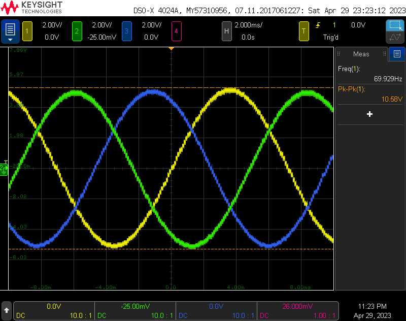
Three-phase power supply output at 100% RPM.
To test the software and hardware, I powered up the boards using a bench supply, connected the Pico’s serial port to a PC, and connect the board’s outputs to three channels on oscilloscope. I entered 100% and captured the image above on the oscilloscope. It shows three 70 Hz signals at 10.58 Vpp and separated by 120°.
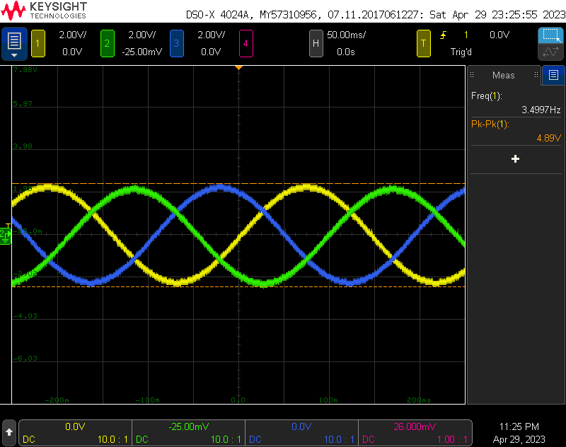
Three-phase power supply output at 5% RPM.
I repeated this procedure at several other percent max RPM values. At 5% max RPM, the frequency was down to 3.5 Hz and the voltage was down to 4.59 volts as shown in the scope traces above.
| Percent Max RPM | Expected Frequency | Expected Voltage | Measured Frequency | Measured Voltage |
|---|---|---|---|---|
| 120% | 84.0 Hz | 10.16 Vpp | 84.032 Hz | 10.58 Vpp |
| 105% | 73.5 Hz | 10.16 Vpp | 73.736 Hz | 10.51 Vpp |
| 100% | 70.0 Hz | 10.16 Vpp | 69.929 Hz | 10.51 Vpp |
| 75% | 52.5 Hz | 10.16 Vpp | 52.492 Hz | 10.58 Vpp |
| 50% | 35.0 Hz | 8.30Vpp | 35.034 Hz | 8.57 Vpp |
| 25% | 17.5 Hz | 6.18 Vpp | 17.520 Hz | 6.56 Vpp |
| 5% | 3.5 Hz | 4.49 Vpp | 3.4997 Hz | 4.59 Vpp |
| 0% | 0 Hz | 0 Vpp | 0 Hz | 0 Vpp |
The results of all my measurements are summarized in the table above. The measured frequencies and voltages were all within an acceptable margin of error of the expected values.
| Percent Max RPM | Measured Current |
|---|---|
| 120% | 72 mA |
| 105% | 79 mA |
| 100% | 82 mA |
| 75% | 108 mA |
| 50% | 110 mA |
| 25% | 100 mA |
| 5% | 81 mA |
| 0% | 20 mA |
Convinced the power supply was working, I attached the tachometer to the power supply and powered it up then measured the current pulled by my three phase-power supply from the bench supply at the same percent max RPM values. These results are shown in the table above.
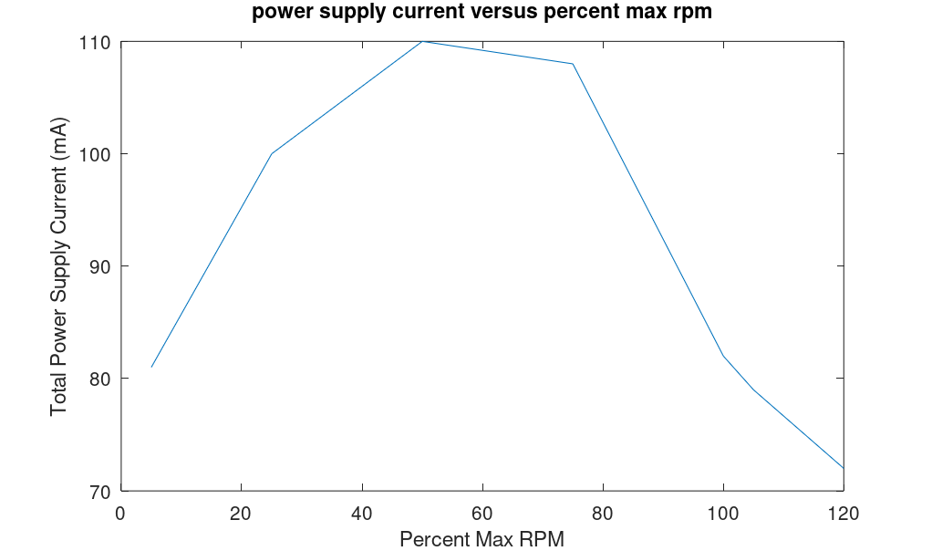
Plot of the total power supply current versus the percent max RPM for the tachometer.
I plotted these values in the graph above. The power supply current increases from 0% peaking at 110 mA at 50% then declined t0 72 mA at 120% max RPM.
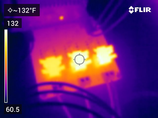
A FLIR image of the buffers with their heatsinks with the tachometer running at 50%. They’re a bit warm but seem to be holding up OK.
The image above is a thermal photo of the LT1010 buffers and their heat sinks after several minutes of operation at 50% max RPM. They’re warm but seem to be holding up OK. The DIP-8 package is not very thermally efficient. If I needed more current, I could move to a more thermally efficient package or move to a purpose-designed power op amp.
Measuring the Speed of the Motor
An animation constructed from 27 frames of the video which was shot at 240 fps, 1/1000 s, f/4, and 12 dB gain. The video was used to measure the RPM of the tachometer’s motor.
One question that had been lingering in the back of my mind was if the tachometer’s motor was really spinning at 4200 rpm with a 70 Hz input. If the motor only had two poles, this would indeed be the case. But nothing says the motor has to have two poles so I devised an experiment to measure the speed of the tachometer motor and thus determine the number of poles.
I focused a video camera shooting at 240 fps (actually 239.76 fps) in 1080p on the end of the magnetic drum with the copper drag cup and dial indicators removed. I set the camera for 1/1000 second shutter speed, f/4, and 12 dB of gain. I used a bright, non-flickering LED light to illuminate the magnetic drum. I fed a 17.5 Hz signal to the tachometer motor which corresponds to a reading of 25% of maximum RPM. I then filmed the rotating magnetic drum for several seconds.
Once the filming was complete, I loaded the footage into Final Cut Pro and scrubbed back and forth to count the number of frames required for the magnetic drum to make one complete revolution. A frame from the captured footage is shown above. It took 28 frames at 239.76 fps for the drum to make one complete revolution. This works out to 8.5629 revolutions per second or 513.77 RPM.
This is approximately 525 RPM which is what a four-pole motor would produce at 17.5 Hz. From this experiment, I concluded that the tachometer’s motor is a four-pole motor. If you look closely at the earlier photo of the disassembled motor, you can see 12 coil groups. 12 coil groups divided by three phases is four poles thus further confirming it is a four-pole motor.
A four-pole motor like this one will spin at a speed of 2100 RPM with a 70 Hz input so it’s spinning at 2100 RPM at 100%; not 4200 RPM. Keep in mind this is just the speed of the motor internal to the tachometer indicator that produces a 100% of max RPM reading with a 70 Hz AC input. This is not the speed of the engine or generator at 100% of max RPM.
If I had access to a stroboscope possibly like an old car timing light, this measurement would probably be a bit more exact but counting the number of video frames is sufficient given that the number of poles has to be an even positive integer.
Displaying PC CPU Usage on the Tachometer
A video showing the Kollsman electric tachometer indicator used as a percent CPU utilization indicator under Windows 10 while running Autodesk Fusion 360.
In the video above, I use a C# console app to get the percent CPU utilization from Windows and send the percent utilization to the power supply board. The percent utilization is then displayed by the tachometer indicator.
The video shows a few windows running on my computer with an inset video overlay showing the tachometer indicator. The upper right window is the Windows Task Manager open to the performance tab and showing the CPU load. The window below that is the console application showing the value of the CPU load from a System.Diagnostics.PerformanceCounter object that is sent to the power supply board and tachometer.
To the left of those windows, I launch Autodesk Fusion 360, open a design, orbit the design around, then render it. As I complete various tasks in Fusion 360, the CPU load varies considerably. The Task Manager, console app, and tachometer indicator all track the CPU load. The tachometer indicator is a mechanical device so it may not indicate the peak load if the duration of the peak is too short for it to spin up to the peak level.
Bonus Content
Flying at Night
A quick turn with a screwdriver permits removal of the lamp holder and lamps for changing the bulbs.
This indicator has lamps in the housing to illuminate the dials at night. Unlike many other aircraft indicators that require removal and disassembly of the indicator to relamp them, this indicator has two small lamp holders with bayonet fittings that permit relamping without removal or disassembly.
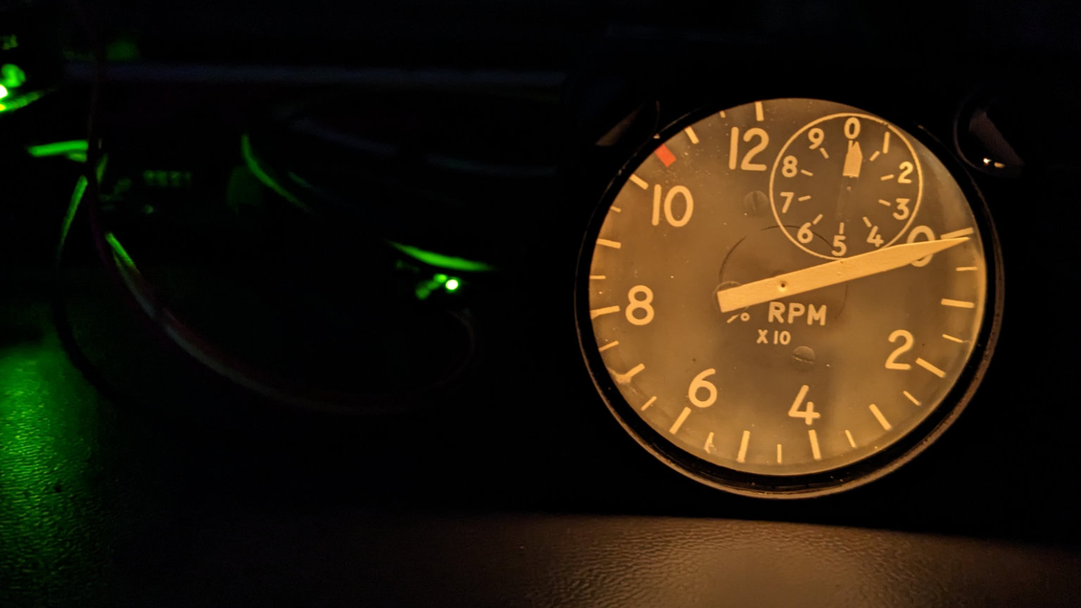
The tachometer with the front illumination turned on.
The bulbs are ordinary 328 miniature bulbs with midget flange bases. They’re 6 volt, 0.2 amp, 1.2 watt T1-3/4 lamps. The two lamps are connected in parallel directly to the two lamp pins on the rear connector. The indicator looks pretty good at night!
Rear Connector Pinout
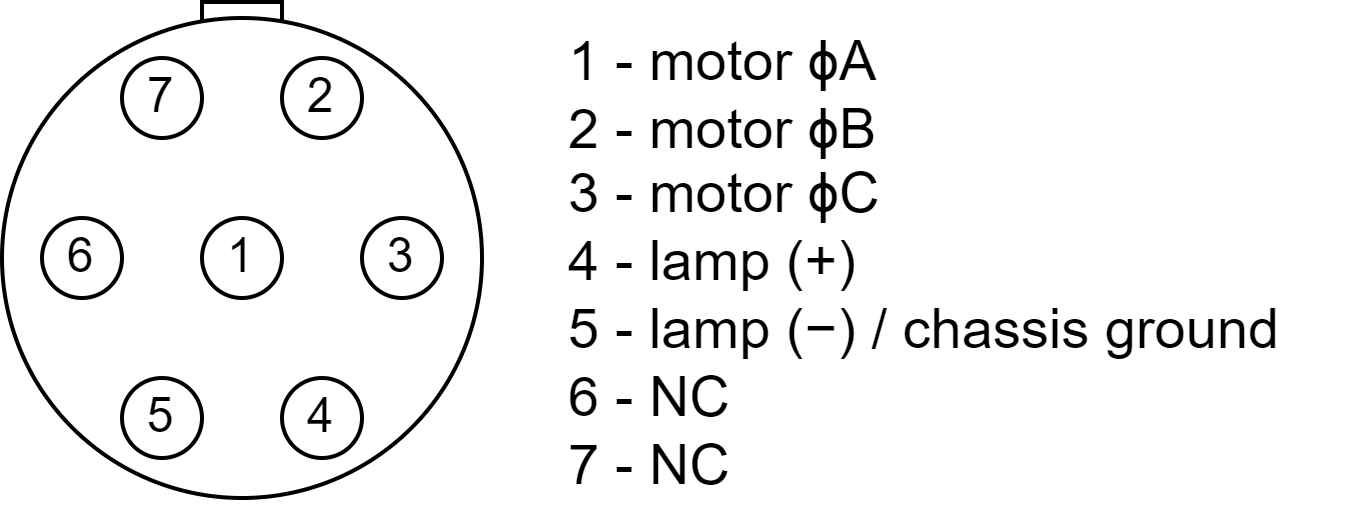
The pinout of the tachometer. This is looking into the receptacle from the rear of the unit.
The pinout of the tachometer is as follows:
1 – motor ϕA
2 – motor ϕB
3 – motor ϕC
4 – lamp (+)
5 – lamp (−) / chassis ground
6 – NC
7 – NC
The pin numbers are visible inside the connector shell.
Related Patents
US Patent 1,309,390 from 1919. Copper lip (25) on copper bowl (2) spun between magnets (19) causing a force to be exerted on shaft (8) counter to the force exerted on the shaft by hairsprng (20) causing pointer (8) to indicate the speed of the bowl.
The earliest patent I could find related to using magnets, copper, and Eddy currents dated from 1919. It concerned the use of a tachometer to optimize the separation of cream from milk. A lip on a copper bowl spun between two magnets. The two magnets were attached to a hairspring and pointer. When the bowl was spinning at the optimal speed for separating the cream from the milk, the pointer would be centered on the scale.
Check it out: Electromagnetic speed-indicator for cream clarifiers and separators.
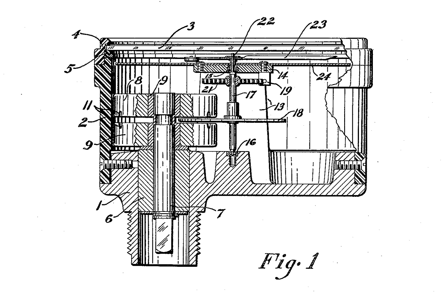
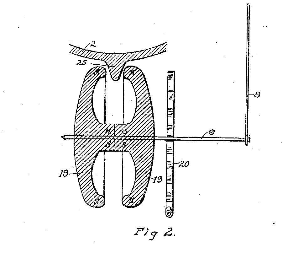
US Patent 2,593,646 from 1946. Magnetic discs (8) and (9) spin on shaft (7) inducing an Eddy current in highly-conductive disc (18) causing a force to be exerted on shaft (17) counter to the force on the shaft by hairspring (21) causing pointer (23) to indicate the shaft’s (7) speed on dial (24).
Another interesting patent is US2593646A for a magnetic drag tachometer filed by the Kollsman Instrument Corporation. This patent was the earliest I could find for a general purpose magnetic drag tachometer indicator. The tachometer in this patent uses a highly conductive disc sandwiched between two rotating magnetic discs rather than a magnetic drum and conductive cup like the tachometer examined in this post.
Final Thoughts
I’d always wondered how a tachometer or a speedometer converted a rotation into an indication of RPM or speed without spinning the needle off the dashboard. Digging into this aircraft tachometer answered that question. This indicator was truly a piece of precision engineering and likely state of the art in its day. The use of Eddy currents to exert a drag force on a shaft connected to a needle and the use of AC synchronous machines to transmit the rotation from a generator to the indicator were both ingenious.