

Can this hardware determine the angle of the fine altitude’s synchro resolver accurately? Read on to find out!
This project uses modern data acquisition hardware to track the shaft angle of a synchro transmitter as the shaft is turned through various angles. How difficult could it be to get the absolute angle of a position sensor from the 1980’s that was originally developed during the WWII era into a modern computer? Turns out, it’s more difficult than it seems, and for most hobbyist applications, more difficult than it’s worth. Read on to find out more.
Encoders and Potentiometers and Synchros! Oh My!
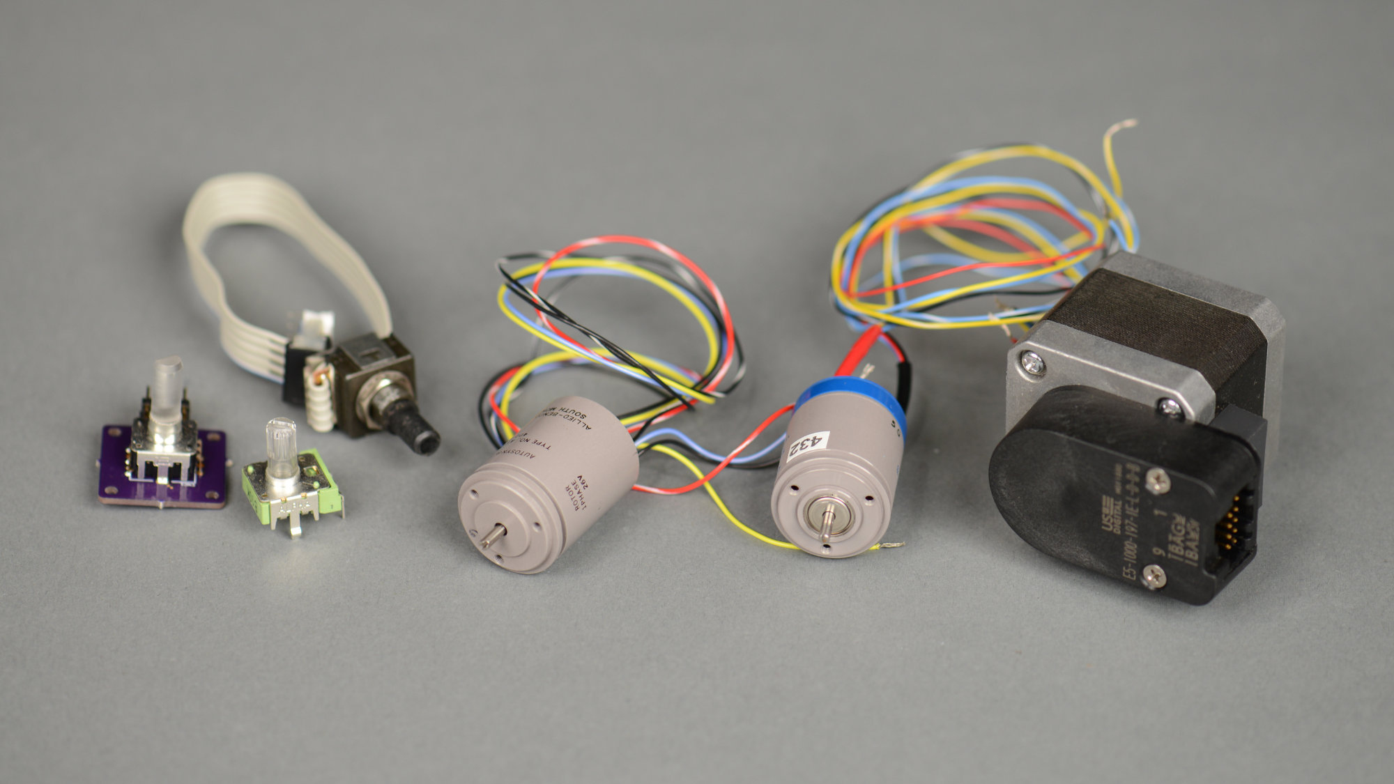
A variety of rotation / angle sensing devices. From left to right: a mechanical encoder, a potentiometer, an optical encoder, a synchro transmitter, a differential resolver, and an optical encoder mounted to the rear of a stepper motor.
The synchro, like a potentiometer or encoder, is a device for converting a mechanical rotational position into an electrical signal representing that position or a change in that position.
Potentiometers are inexpensive and easy to interface to micros with ADCs. Encoders range from inexpensive, crude mechanical incremental encoders to expensive, precision optical absolute encoders. Encoders have digital outputs and are easy to interface to micros too.
Synchros, on the other hand, can be expensive and require the user to generate and process AC waveforms. Synchros have several advantages over their more common counterparts that might lead one to choose a synchro instead of potentiometer or encoder:
- Synchros always provide the absolute position of the mechanical shaft without requiring a homing sequence.
- Even basic synchros have precision and accuracy measured in arc minutes. Only high-end absolute position optical encoders can come close to synchro’s resolution.
- Synchros have ratiometric outputs that provide high noise immunity.
- Synchros are transformers and thus inherently provide galvanic isolation and high common-mode rejection of interference.
- Synchros are more reliable than potentiometers and encoders.
The major downsides of a synchro:
- Synchros are expensive but they’re still less than an absolute optical encoder with the same precision.
- Synchros are transformers and thus only work with AC signals.
As a result, synchros tend to be used mostly for military, aerospace, industrial, and automotive applications that demand their precision, accuracy, and reliability.
Synchro Transmitter Basics
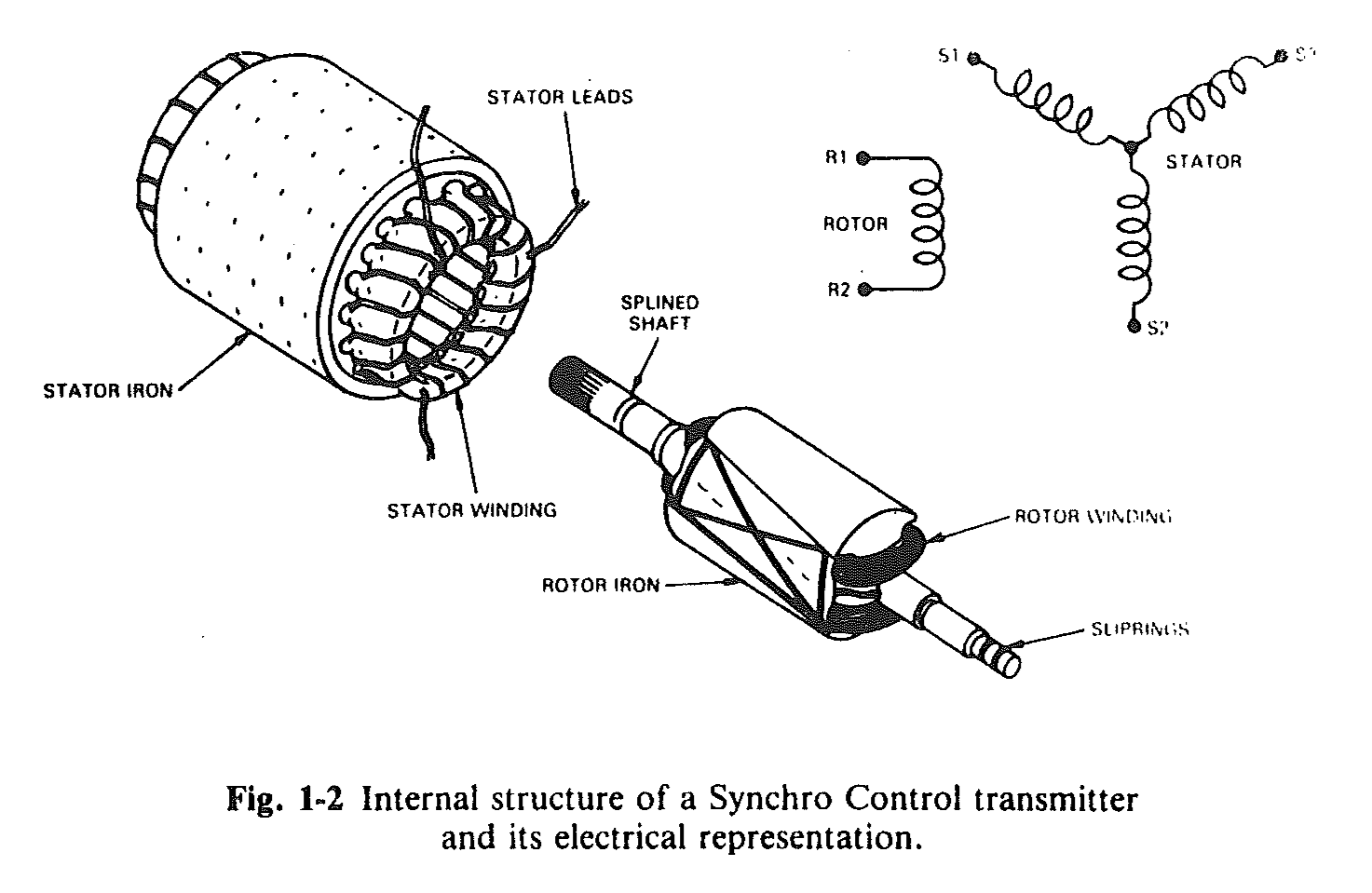
Internal structure of a synchro control transmitter and its electrical representation from the Analog Devices Synchro and Resolver Conversion Handbook.
The Analog Devices Synchro and Resolver Conversion Handbook is a great reference for detailed information on the different types of synchros, resolvers, and control transformers, how they work, and how to build systems from these components. For the purposes of this blog post, only the basics of a synchro transmitter need to be understood and we’ll briefly cover those here. The figure above is a schematic representation of a synchro transmitter from the handbook.
The synchro transmitter is essentially a single-phase to three-phase transformer in which the single-phase primary rotor winding is free to rotate within the stationary three-phase secondary stator windings and the voltage transferred between the primary winding and the secondary windings is proportional to the cosine of the angle between the primary coil axis and each of the secondary coils’ axes.
Mathematically speaking, if the rotor is excited by applying a reference AC voltage across the two rotor terminals of the form:
Vref = VR2 – VR1 = A ⋅ sin ωt
The synchro transmitter will develop voltages across the three stator terminals of the form:
VS1 – VS3 = k ⋅ A ⋅ sin ωt ⋅ sin θ
VS3 – VS2 = k ⋅ A ⋅ sin ωt ⋅ sin (θ + 120°)
VS2 – VS1 = k ⋅ A ⋅ sin ωt ⋅ sin (θ + 240°)
where θ is the synchro shaft angle and k is the coupling transformation ratio.
The coupling transformation ratio is the ratio of the maximum output voltage to the maximum input voltage and is determined primarily by the ratio of the number of windings in each coil. As we’ll see later, it’s possible to recover the shaft angle, θ, given the four voltages.
Synchros can be designed to run at any voltage and frequency but most of them are designed for 115 VAC / 60 Hz or 26 VAC / 400 Hz operation. The 26 VAC / 400 Hz synchros usually have a secondary of 11.8 VAC. In the case of a 26 VAC / 400 Hz synchro, the values in the equations above then become:
A = 26 ⋅ sqrt (2) = 36.77 volts
ω = 2πƒ = 2π ⋅ 400 = 2513.3 rad/sec
k = 11.8 / 26.0 = 0.45385
Selecting and Using a Synchro Transmitter
Selecting the Synchro
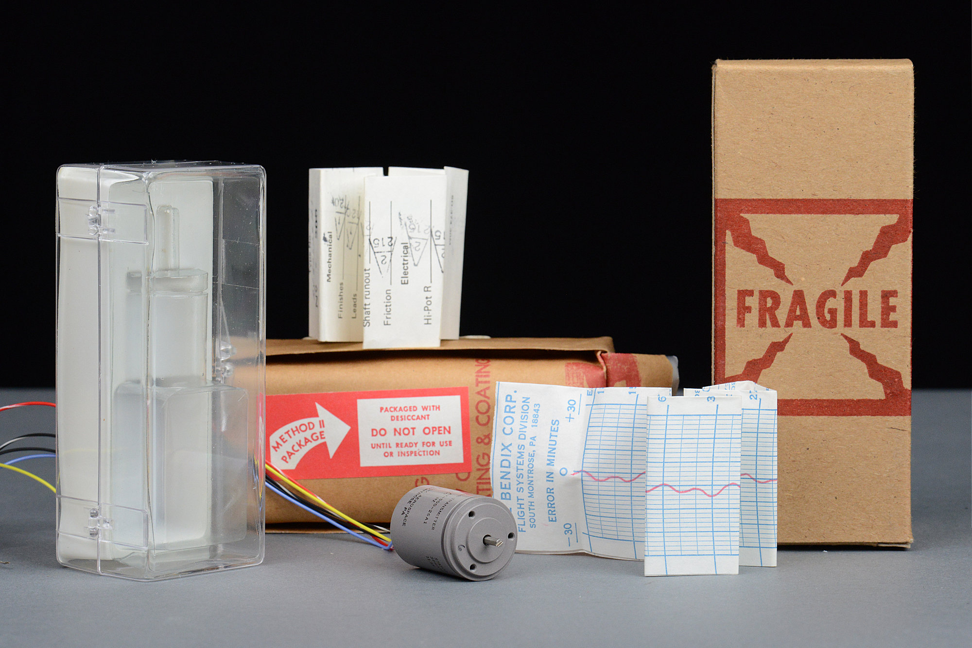
My Bendix Autosyn AY-500-26A1 synchro transmitter, its packaging, and its individual test results.
Armed with a little bit of knowledge, I headed to eBay to find a suitable synchro transmitter. Rather than risk a painful death by electrocution, I quickly scratched 115 VAC / 60 Hz synchros off the list and focused my search on 26 VAC / 400 Hz synchros. After searching for a bit, I found one with a 26 VAC single-phase rotor and an 11.8 VAC three-phase stator designed for operation at 400 Hz and at a reasonable price. It’s pictured above with its packaging and individual test results.
26 VAC is 73.5 VPP which is still high. Fortunately, synchros are magnetic components and will run at lower voltages but with reduced performance. In the case of a high-impedance load like a synchro-to-digital converter, the reduced performance won’t matter too much. In the case of a low-impedance load like a synchro receiver, the performance may be reduced too much for the system to work.
Identifying the Leads
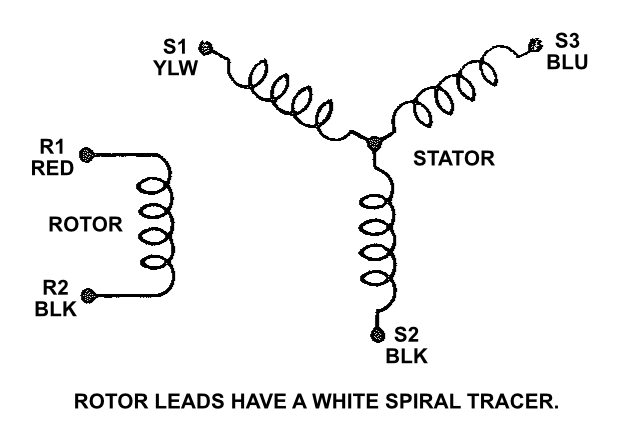
The terminal numbers and lead colors for my synchro transmitter.
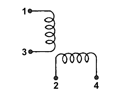
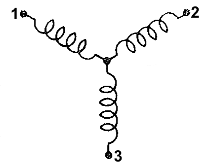
Datasheets for most synchros have been lost to the dustbin of history. Fortunately the terminal numbering and lead color coding seems somewhat standardized. The number of terminals and leads depends on the number of phases on the rotor and the number of phases on the stator. The table below shows the terminal numbers and lead colors for the rotor and stator based on the number of phases.
| Phases | 1 | 2 | 3 |
| Terminals / Leads | 2 | 4 | 3 |
| Schematic | 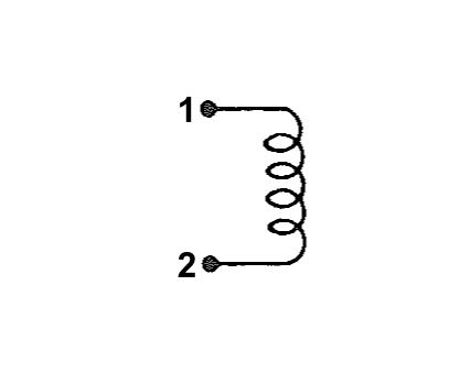 |
 |
 |
| Rotor Terminal Numbers and Lead Colors* | R1 – Red R2 – Black |
R1 – Red R3 – Black R2 – Yellow R4 – Blue |
R1- Yellow R2 – Black R3 – Blue |
| Stator Terminal Numbers and Lead Colors | S1 – Red S2 – Black |
S1 – Red S3 – Black S2 – Yellow S4 – Blue |
S1- Yellow S2 – Black S3 – Blue |
| *Rotor leads have a white spiral tracer. | |||
Both the rotor and stator leads use the same color codes except that the rotor leads have white spiral tracers on them while the stator leads are uniform in color.
My synchro transmitter has red and black leads with a white spiral tracer so those are the R1 and R2 rotor leads respectively. It also has solid yellow, black, and blue leads so those are the S1, S2, and S3 stator leads respectively. The next step was to hook up the synchro and verify it works as expected.
Testing it Out
Synchro transmitter voltages with a shaft angle of 0°.
The figure above shows the operation of the synchro transmitter with an approximately 6.5 VAC (18 VPP) reference voltage and the shaft angle at 0°. The four traces in order are VR2 – VR1, VS1 – VS3, VS3 – VS2, and VS2 – VS1. The reference voltage was generated using a homemade function generator (to be described later) set for 18 VPP and 400 Hz. The traces were captured using a data acquisition device with differential inputs (also to be described later).
Note that at 0°:
VS1 – VS3 is roughly 0.0 VPP
VS3 – VS2 is in-phase with the reference voltage and is roughly 7.0 VPP
VS2 – VS1 is out-of-phase with the reference voltage and is roughly 7.0 VPP
This is exactly as predicted by the stator voltage equations in the previous section.
Synchro Transmitter Internal Photos
While collecting the above data, I snapped the black with white spiral tracer rotor wire off the synchro transmitter. With nothing to lose, I disassembled the synchro and was able to repair it. While it was a part, I took a few photos of its construction. Soldering the rotor’s wire back to the brush turned out to be a relatively simple repair. A repair to a stator winding wire, however, would not have been possible. I got lucky.
Here’s a photo of the rotor:
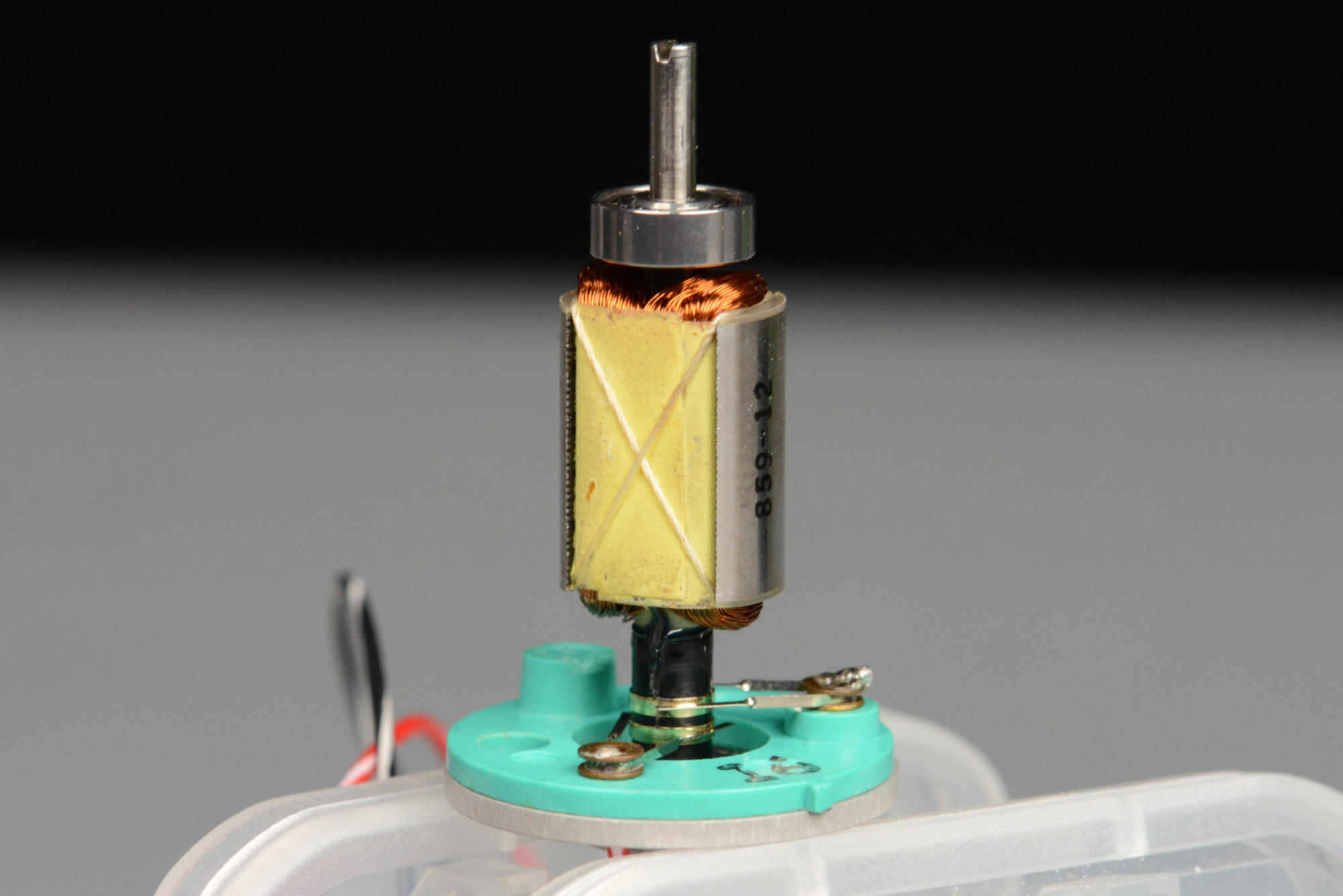
The synchro’s single phase rotor winding, shaft, bearings, slip rings, and brushes.
Note that the brushes operate on continuous slip rings rather than segmented surfaces like in a brushed motor. The continuous rather than segmented nature of the brush contact surfaces contributes to the reliability of synchros versus a brushed motor.
And here’s a photo of the stator:
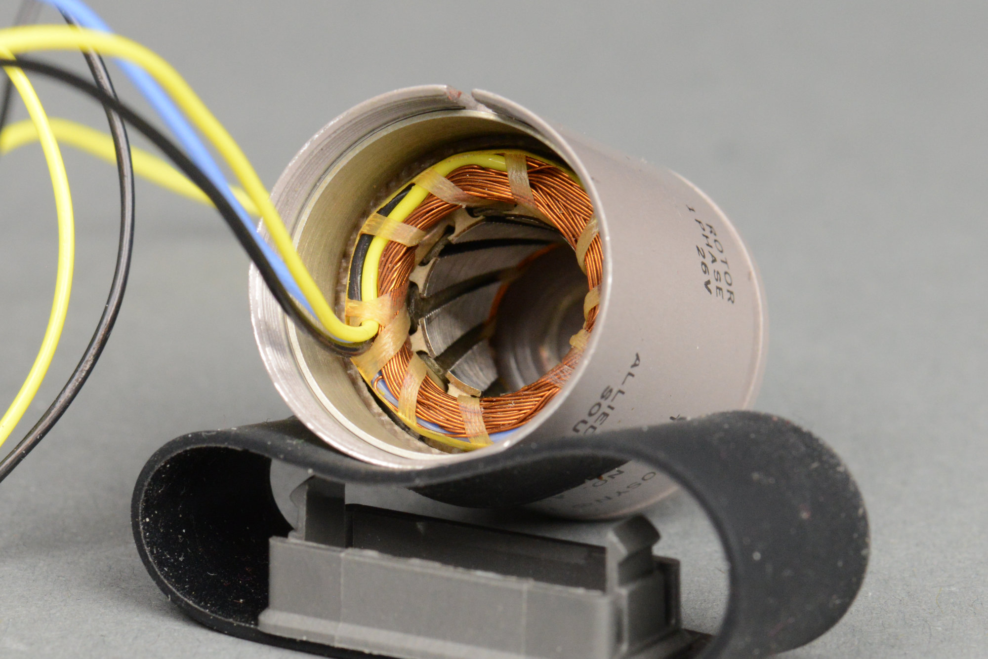
The synchro’s three phase stator winding.
With repairs complete and the synchro reassembled, it was time to continue the project.
Modeling a Tracking Synchro-to-Digital Converter
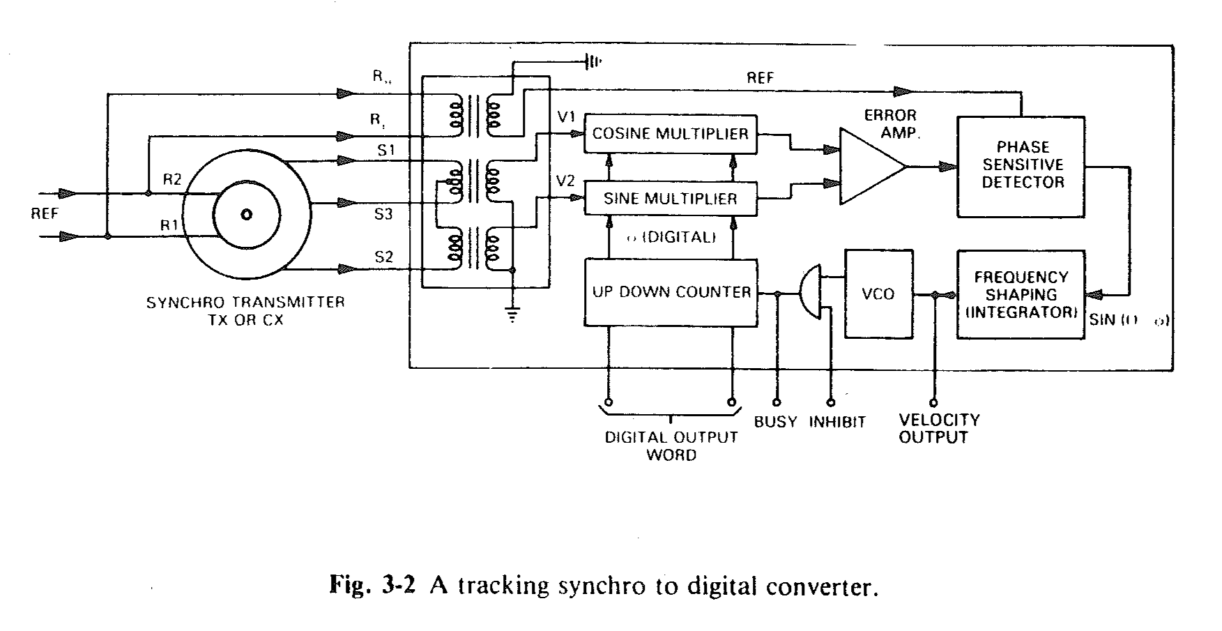
A tracking synchro to digital converter from the Analog Devices Synchro and Resolver Conversion Handbook.
The figure above shows a block diagram of a tracking synchro-to-digital converter from chapter three of the Analog Devices Synchro and Resolver Conversion Handbook. Using this diagram, the handbook explains the math used to calculate the digital output word using the reference voltage input and synchro format voltage inputs.
While it would be possible to build a synchro-to-digital converter using the combination of analog and digital parts and techniques shown in the block diagram above and described in detail in chapter three, the tracking loop can be implemented much more efficiently in software today.
Before getting started with real hardware, I decided to model a synchro transmitter and a synchro-to-digital converter in GNU Octave. This would let me ensure my math and logic were correct before committing to buying or building hardware.
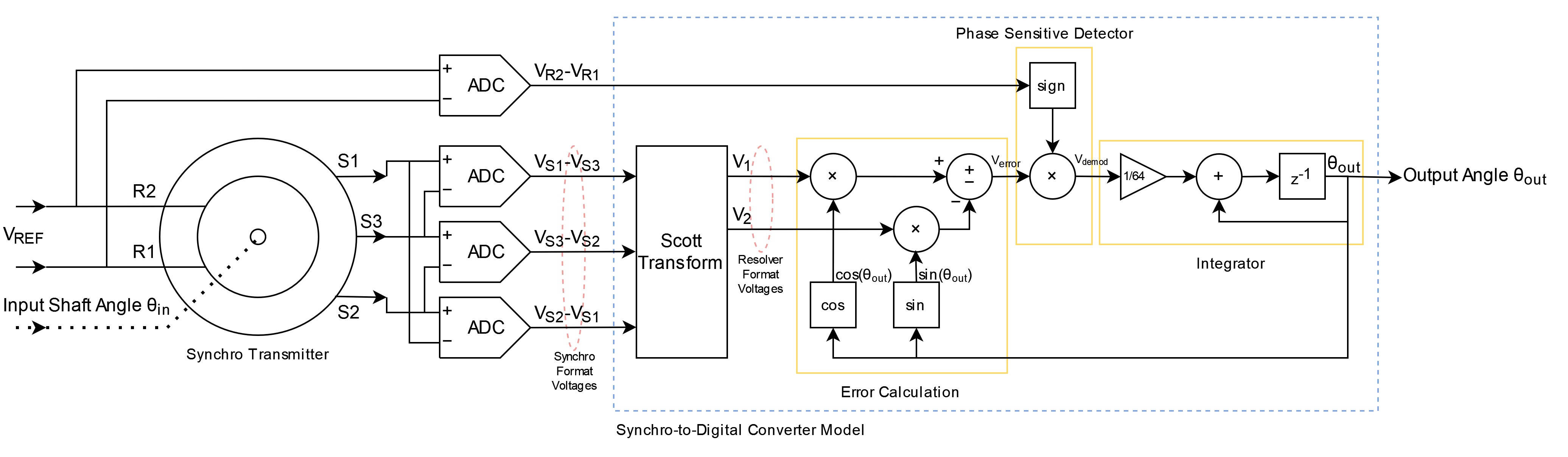
Block diagram of the system to model.
After studying chapter 3 of the handbook, I came up with the block diagram shown above for a DSP implementation. The system consists of a synchro transmitter connected to a tracking synchro-to-digital converter . The inputs to the system are the AC reference voltage and the input shaft angle, θin. The output from the system is the computed output angle, θout.
The inputs to the synchro-to-digital converter model are the reference voltage, VR2-VR1, and the three synchro format voltages from the synchro transmitter, VS1-VS3, VS3-VS2, and VS2-VS1. In a system built using real hardware, the inputs to the converter would be digitized using ADCs with differential inputs. In the model, they’re just the outputs from the synchro transmitter model.
With that said, let’s dig in to the code. The code sets up some variables that will be used later, creates a time vector with all the time steps we’ll process in the model, and then creates the 400 Hz AC reference voltage input vector, ref, with an amplitude of 1 volt:
# setup
length=25e3/40e3;  # time in seconds
Fs=40e3;        # sample rate
T=1/Fs;         # period

# create time vector
t=0:T:length;

# create reference waveform
ref = sin (2*pi*400*t);
Figure 1 below is a plot of the reference voltage versus time as a sanity check. The model runs for 0.625 seconds and the reference voltage has an amplitude of 1 volt and a frequency of 400 Hz.
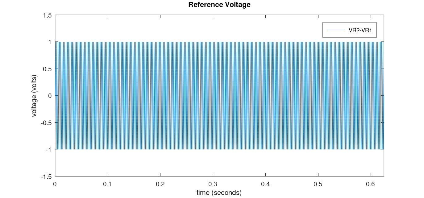
Figure 1.
The next step is to create the vector setpts containing the input shaft angles in radians over time:
# create set points
setpts = zeros (size (t));
setpts(    1:5000) = -90;
setpts( 5001:10000) = -90:90/5000:-90/5000;
setpts(10001:15000) = 0;
setpts(15001:20000) = 0:90/5000:90-90/5000;
setpts(20001:25000) = +90;
setpts(25001) = +90;
setpts = setpts * pi/180;
With the reference voltage and input shaft angles defined, we can model the synchro transmitter and create the three synchro format voltages, s1ms3, s3ms2, and s2ms1. The variables ref, s1ms3, s3ms2, and s2ms1 are the inputs to the synchro-to-digital converter model. One side note is that the s2ms1 input is never actually used.
# create synchro waveforms
s1ms3 = ref .* sin (setpts);
s3ms2 = ref .* sin (setpts + 120*pi/180);
s2ms1 = ref .* sin (setpts + 240*pi/180);
The converter works using resolver format voltages so the next step is to convert the synchro format voltages to resolver format voltages using the Scott transform. The Scott transform is the first processing block inside the converter model. The output of the Scott transform is the resolver format voltages, sinin and cosin, which are of the form:
sinin = (VR2-VR1) ⋅ sin θin = s1ms3
cosin = (VR2-VR1) ⋅ cos θin = 2/sqrt(3) ⋅ (s3ms2 + 0.5 ⋅ s1ms3)
# create sin and cos inputs using scott transformation
sinin = s1ms3;
cosin = 2/sqrt(3) * (s3ms2 + 0.5 * s1ms3);
The three plots in Figure 2 below shows the input shaft angle, the corresponding synchro format voltages, and the corresponding resolver format voltages. Note that both the synchro and resolver format voltages are 400 Hz AC waveforms with amplitudes dependent on the input shaft angle.

Figure 2.
Next up is to model the error calculation, demodulate the AC error term, and integrate the demodulated AC error term into the output angle. The code only needs the sign of the reference waveform for the phase sensitive detector:
# convert ref waveform into square waveform
refsq = sign(ref);
The code initializes the output state vector, theta, to 0. The vector theta is the computed output angle, θout. It also creates the zero vectors delta and demod to save intermediary values for plotting later. In a real system, these would all be scalar variables and the intermediary values would not be saved.
# init state variables
theta = zeros(size(t));
delta = zeros(size(t));
demod = zeros(size(t));
Run a loop over the input data to calculate the output data:
for i=1:size(t)(2)-1
The following code calculates the error, delta, between the input signals, sinin and cosin, and the present value of the output angle, theta. The details of this calculation are in chapter 3 of the handbook on page 46. The net result is to produce an AC modulated signal whose amplitude is proportional the error between the input shaft angle, θin, and the computed output shaft angle, θout:
delta = sin ωt ⋅ sin (θin – θout)
  # calculate AC error term
  delta(i) = sinin(i)*cos(theta(i)) - cosin(i)*sin(theta(i));
The phase sensitive detector sounds complicated but all that’s required is to multiply the error by the sign of the reference voltage. If I remember correctly what I read somewhere, this works well for phase differences of up to about ±20° without any issues. This produces a DC error signal that is proportional to the difference between θin and θout:
demod = sin (θin – θout)
  # demodulate AC error term
  demod(i) = refsq(i) * delta(i)
The last calculation step is to integrate and to wrap the angle so that it is always between -π and +π. The demodulated error term is scaled by 1/64 before integrating. This value seemed to work pretty well in the model.
  # apply gain term to demodulated error term and integrate
  newtheta = theta(i) + 1/64*demod(i);

  # wrap from -pi to +pi
  theta(i+1) = mod(newtheta+pi, 2*pi)-pi;
Finally, finish the loop:
endfor
Figure 3 below shows the error, demodulated error, input shaft angle, and computed output shaft angle from the entire run of the simulation.
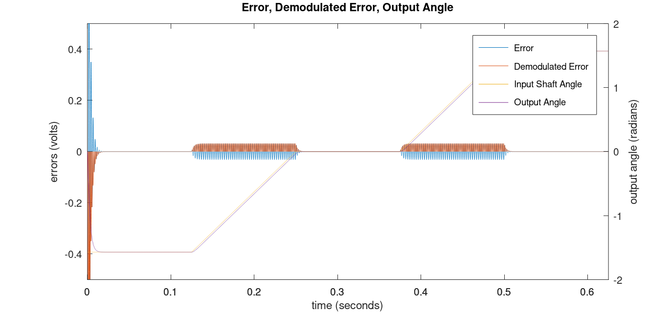
Figure 3.
Figure 4 is a close up of the region from 0.1 to 0.275 seconds. The error signal in blue is an AC waveform. Attempting to integrate this signal would result in an output angle that never changes because the DC value is 0. The demodulated error signal in red orange, however, has a DC value.
In this case, the DC value is positive because the output angle is lower than the input shaft angle. Integrating this value will cause the output shaft angle value to increase until the error is zero. If the error were in the other direction, the red orange demodulated error signal would be negative instead of positive and the integrated value would decrease.
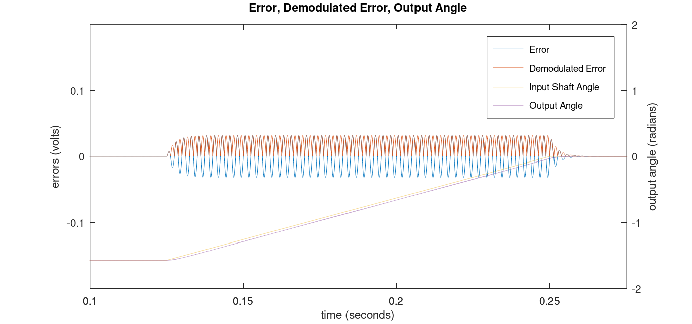
Figure 4.
Figure 5 below shows the input shaft angle versus the computed output angle. This looks pretty good to me and I have high confidence my synchro-to-digital converter will work when implemented using real hardware and this algorithm.
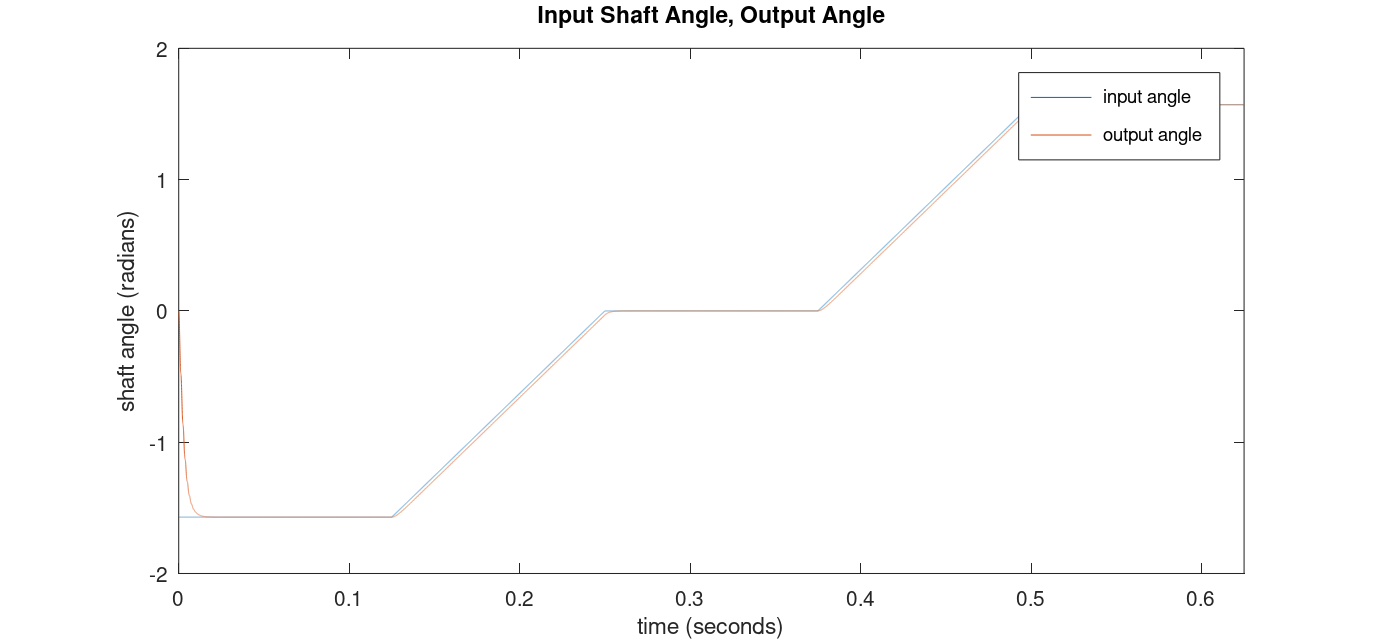
Figure 5.
The complete code for the Octave simulation of the tracking synchro-to-digital converter without the annotations and with the code to generate the five plots can be downloaded from the download links at the end of this post.
Constructing a Reference Voltage Source
With the modeling completed, it was time to build a reference voltage source to power the synchro. This synchro requires a 26 VAC 400 Hz power supply. 26 VAC works out to 73.5 VPP. This is well outside the capabilities of my bench supplies and also well outside my area of expertise. From some experiments with a function generator, the synchro transmitter, and some low-cost data acquisition hardware (described in next section), the hardware appeared to work well enough from 20 VPP which is only 7.1 VAC.
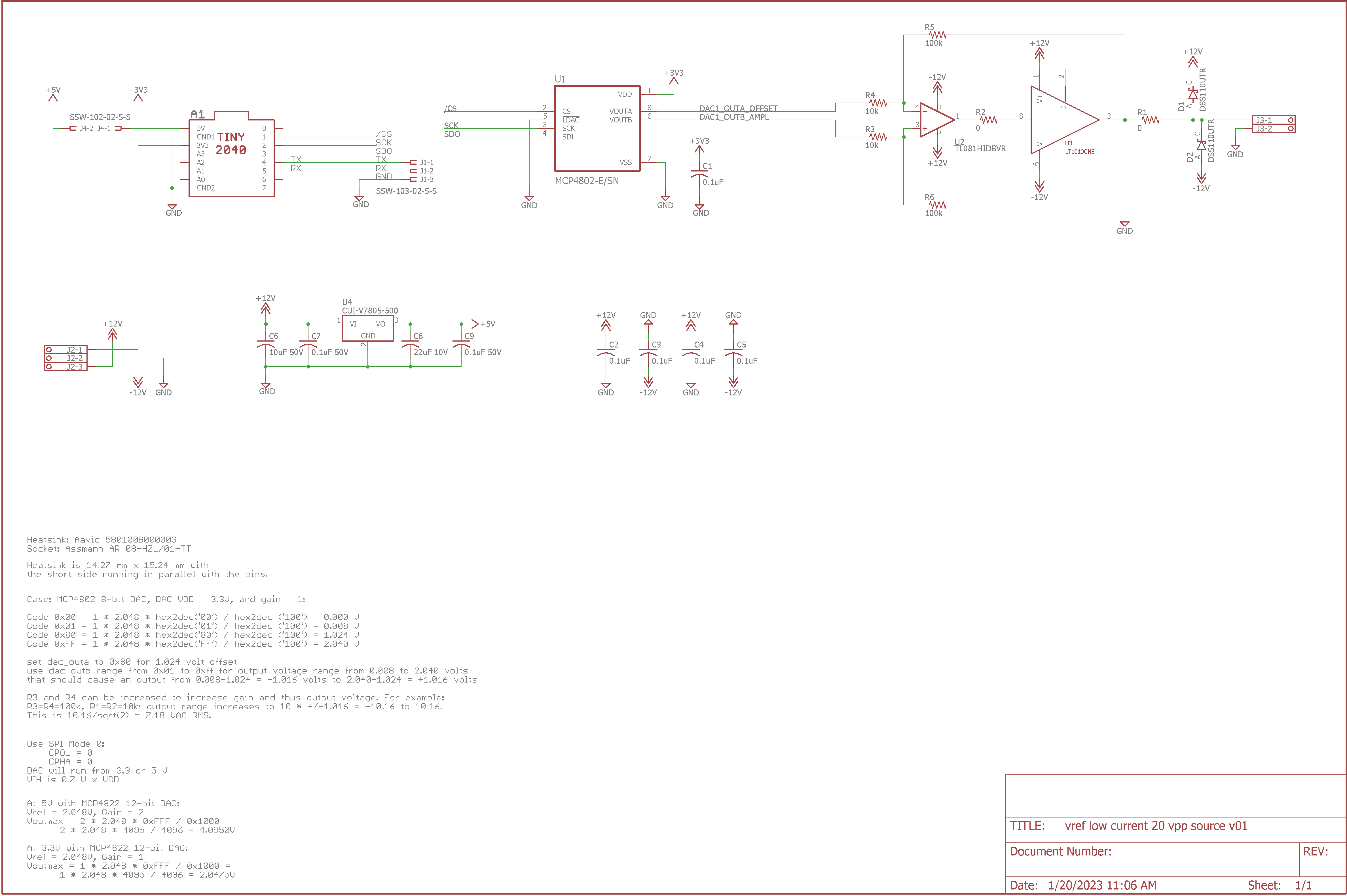
Schematic of the synchro reference voltage generator.
The schematic above shows the reference voltage source design. It’s a programmable arbitrary waveform generator with a maximum output of 20 VPP / ±10 V. It’s capable of driving a few 10’s of milliamps into a load without going up in flames.
Software running on the Pimoroni Tiny 2040 uses a lookup table to send a 400 Hz sine wave sampled at 40,000 kHz over the SPI bus to a Microchip MCP4802 8-bit DAC. Channel A of the DAC is fed to the inverting input of an opamp and is used as a reference voltage to control the voltage offset of the sine wave. Channel B of the DAC outputs the sine wave and is connected to the non-inverting input of the opamp. The opamp’s gain is 10. An Analog Devices LT1010 Fast ±150mA Power Buffer is used in the opamps’s negative feedback loop to increase the drive strength of the circuit. The circuit is powered from a ±12 V bench supply. An on-board DC/DC switching regulator is used to supply +5 V to the Tiny 2040. 3.5 mm pitch Phoenix Contact rising cage clamp terminal blocks are used for all inputs and outputs.
The 8-bit DAC has a reference voltage of 2.048 V and an internal gain of 1 when running at 3.3 V. At count 1, the DAC outputs 0.008 V and at count 255, the DAC outputs 2.040 V. Supplying only a full-scale sine wave with this voltage range to a non-inverting amplifier with a gain of 10 would result in a 20 VPP sine wave but from 0.080 V to +20.40 V; not ±10 V.
To offset the sine wave to ±10 V, another channel of the DAC is set to mid scale and used as a reference voltage. The reference voltage is applied to the inverting terminal of the opamp and offsets the sine wave downward by the value of the voltage multiplied by the gain. Mid scale is 128 and results in a 1.024 V reference voltage. With the gain applied, this result in a shift of -10.24 V and the sine wave centered on ground from -10.16 V to +10.16 V.
This is close enough to ±10 V for our purposes. We’ll fine tune the voltage slightly in software to keep it within the range of the data acquisition hardware so being precisely ±10 V doesn’t matter.
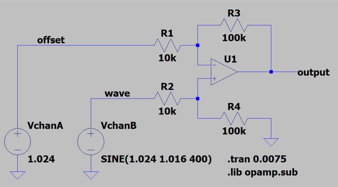
vref gnerator sim schematic
To check the math, I ran a simulation of this circuit in LTSpice. The simulation circuit is shown above. The reference voltage source is a constant 1.024 V. The 400 Hz sine wave voltage source has an offset of 1.024 V, an amplitude of 1.016 V, and extends from 0.008 V to 2.040 V. With these inputs and a gain of 10, the output sine wave should extend from -10.16 V to +10.16 V.
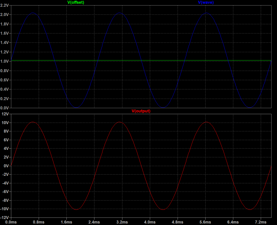
vref gnerator sim outputs
The figure above shows the results of running a transient analysis on the circuit. The top waveform window shows the reference voltage source in green and the sine wave voltage source in blue. These are both positive voltages within the DAC’s output range from 0 V to 2.040 V. The bottom waveform window shows the output voltage in red. The output voltage trace extends from approximately -10 V to +10 V which is the desired output range.
MAX(v(offset))=1.024
MIN(v(offset))=1.024
MAX(v(wave))=2.03889
MIN(v(wave))=0.00800089
MAX(v(output))=10.1469
MIN(v(output))=-10.158
I used the .meas directive in LTSpice to take some measurements from the transient analysis. The measured values are listed above.

Board layout / preview of the synchro reference voltage generator.
The completed board layout is shown above. It’s not the most efficient use of space but I was able to reuse the DAC and analog layout from a previous design which saved some time designing the board.
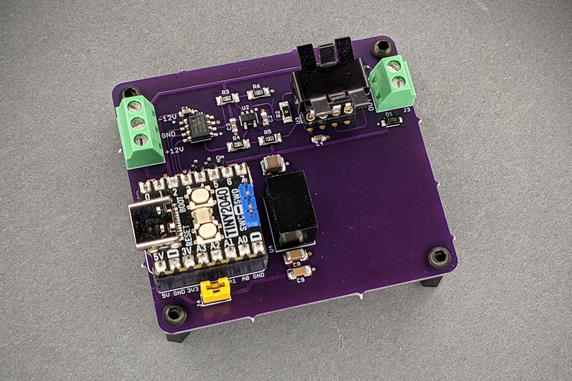
The assembled reference voltage generator circuit board.
When the boards arrived, I stuffed them then hooked them up to develop and test the software. The bench supply connects to the 3 position connector on the left. The synchro connects to the 2 position connector on the right. The jumper connects +5V from the regulator to the Tiny 2040 board. The jumper must be removed if powering the Tiny 2040 from USB. J1 is the RP2040’s UART1 serial port for accessing a small command line interpreter built into the software.
I’m using a Raspberry Pi, OpenOCD, and the SWD interface on the Tiny 2040 board to program and debug the RP2040. One note is that to use OpenOCD with both RP2040 cores running, the OpenOCD command line needs to change versus what’s documented in the RP2040 C SDK getting started documentation:
openocd -f interface/raspberrypi-swd.cfg -f target/rp2040.cfg -c "program sin400.elf verify reset ; init ; reset halt ; rp2040.core1 arp_reset assert 0 ; rp2040.core0 arp_reset assert 0 ; exit"
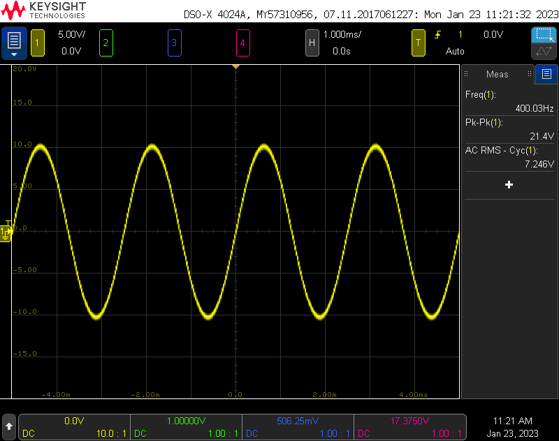
Unloaded reference voltage generator output at 100%.
The figure above is the output of the board running the software with the amplitude at 100% and no synchro connected. The peak-to-peak voltage is 21.4 V and the sine wave is centered at ground with the scope’s coupling set to DC.
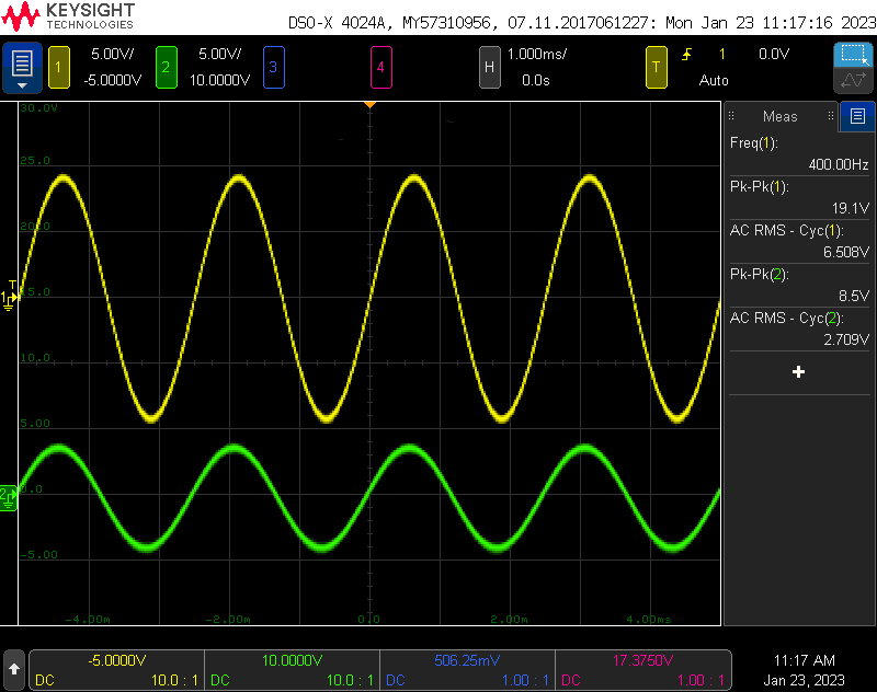
Reference voltage generator output with synchro connected and amplitude adjusted in software to 90% (yellow) and one synchro output with the shaft angle adjusted for maximum output voltage (green).
The figure above has two traces. The yellow trace on channel 1 is the output of the board running the software with the amplitude at 90% and the synchro connected. The peak-to-peak voltage is 19.1 V and the sine wave is centered at ground with the scope’s coupling set to DC. This is ±9.55 V and comfortably within the the input range of the data acquisition hardware. The green trace on channel 2 is the S1-S3 output of the synchro with the shaft angle adjusted to 90° for its maximum voltage output. This is 8.5 V peak-to-peak or ±4.25 V and also comfortably within range of the data acquisition hardware.
Digitizing the Synchro Signals
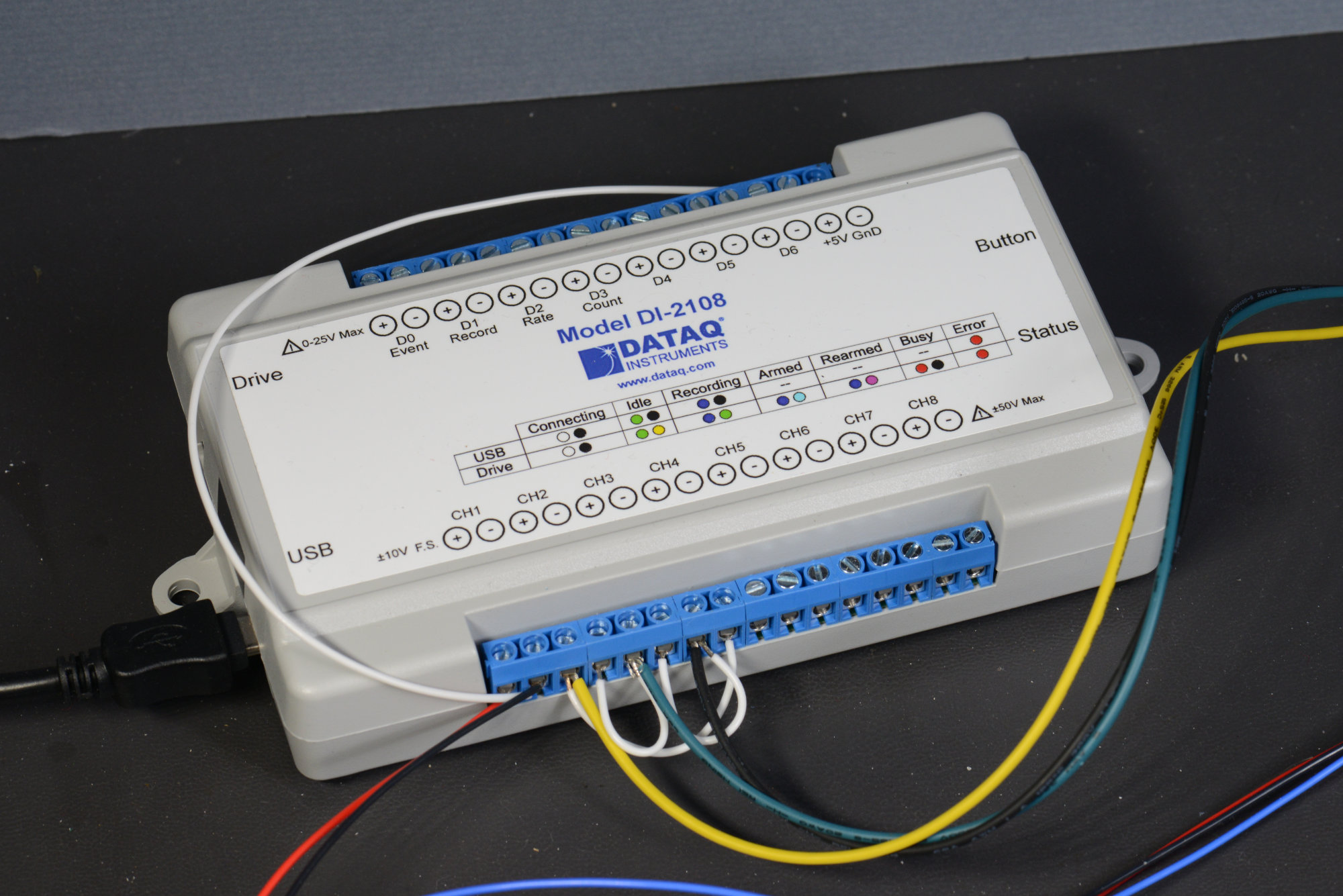
The Dataq Instruments DI-2108 data acquisition hardware. It’s wired up to the reference voltage and synchro voltages. I had to connect the (-) terminal of channel 1 to GND to eliminate 60 Hz noise when using a computer with a floating ground / wall wart power supply.
My primary goal for this project was to see if I could build a synchro-to-digital converter; not to see if I could build an analog data acquisition device. With this goal in mind, I searched for alternatives to building my own hardware. The list of requirements was pretty short:
- 4 input channels.
- 40 kHz sampling rate for each channel.
- ±10 V differential inputs.
- 10-12 bits of resolution.
- Open API.
After examining a bunch of different data acquisition devices from a handful of manufacturers, I found the Dataq Instruments DI-2108. It meets all my criteria, it was in stock, and it was relatively reasonably priced at $199 in late 2022. The only downside is it is USB-only so I’d need to use a PC or microcontroller with USB host capability to acquire and process the data.
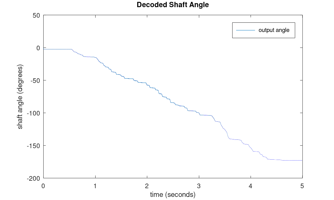
As a quick test of the DI-2108 for this application, I captured the reference and synchro voltages from a synchro transmitter as I turned the transmitter’s shaft slowly by hand. The graph above shows the result of processing the captured data through the synchro-to-digital model.
As a quick test, I hooked up a function generator and the synchro transmitter to the DI-2108. I then captured some data using the included WinDAQ software as I turned the shaft of the synchro transmitter slowly by hand.
I loaded the captured data into Octave and modified the model to process the captured data. The graph above shows the result of processing the data. It shows that I turned the shaft from -2.5° to -173° in five seconds which seems reasonable. This served to validate the Dataq hardware for this application and further validated the synchro-to-digital model.
The included WinDAQ waveform capture software is sufficient for testing connectivity and acquiring data for feeding into Octave as demonstrated above. The real power is the DI-2108 can be switched into USB CDC mode where it appears as a serial device and the open API can be used to configure the instrument and capture data.
Implementing the Tracking Converter
I implemented the tracking synchro-to-digital converter in Python 3.9.5 under Linux Mint 20.1 running on an Intel Celeron J3455 1.5 GHz processor. This is a quick floating-point implementation rather than an optimized fixed-point implementation.
First up is some notes on the reference voltage and synchro are connected to the Dataq hardware. Note that I have the Dataq setup to capture VR1 – VR2 rather than VR2 – VR1 so the channel must be negated later. There’s also a note here about how to offset the angle when using the altitude alerter to make 0° equal 0 feet.
# Connections:
#
# Ch1 is Vr1-Vr2 (red/wht - blk/wht) (from eq set 1)
# Ch2 is Vs1-Vs3 (ylw - blu)         (from eq set 2)
# Ch3 is Vs3-Vs2 (blu - blk)         (from eq set 2)
# Ch4 is Vs2-Vs1 (blk - ylw)         (from eq set 2)
#
# Ch1 needs to be inverted to get the correct angle output
# since Vr1-Vr2 is captured but Vr2-Vr1 is needed.
#
# computing the error as the following results in an angle of 0 at 0 feet on the altitude
# alerter with the angle increasing as the altitude increases:
#     delta = sinin*math.cos(3*math.pi/2 - theta) - cosin*math.sin(3*math.pi/2 - theta)
# this is technically not the correct result but it looks prettier when demoing the system
Python imports:
# imports

import serial
import time
import sys
import struct
import math
Some constants for the serial port with the Dataq and another serial port for displaying the computed output shaft angle. USE_SER_DISP can be set to 0 if the second display serial port is not available or not used.
#----------------------------------------
# constants

DATAQ_SER_PORT = '/dev/ttyACM0' # DI-2108 serial port
DISP_SER_PORT  = '/dev/ttyUSB0' # serial display serial port
USE_SER_DISP   = 1
This function writes a command string to the Dataq then waits up until the timeout time for the command string to be echoed back by the Dataq:
#----------------------------------------
# function to write command to dataq then wait up until the timeout
# for the command string to be echoed back to the hose

def WriteCommandWait (serial, cmd, timeout):
    serial.write(cmd)
    start = time.time ()
    s = b"";
    while not (cmd in s) and time.time () - start < timeout:
        if (serial.in_waiting > 0):
            s = s + serial.read (1)
Open the serial ports:
#----------------------------------------
# open serial ports

serDataq = serial.Serial (port = DATAQ_SER_PORT, timeout=0.5)
if USE_SER_DISP:
    serDisp  = serial.Serial (port = '/dev/ttyUSB0', baudrate = 115200)
Configure the Dataq to capture the first four channels at 40 kHz with no filtering and initialize some local variables. count is used to display the computed output shaft angle at a 100 Hz rate. theta is the computed output shaft angle.
#----------------------------------------
# configure dataq to capture channels 0 to 3 at 40 ksps each

WriteCommandWait (serDataq, b"stop\r", 0.25)      # stop in case device was left scanning
WriteCommandWait (serDataq, b"reset\r", 0.25)     # reset in case of any errors
WriteCommandWait (serDataq, b"encode 0\r", 0.25)  # set up the device for binary mode
WriteCommandWait (serDataq, b"slist 0 0\r", 0.25) # scan list position 0 channel 0
WriteCommandWait (serDataq, b"slist 1 1\r", 0.25) # scan list position 1 channel 1
WriteCommandWait (serDataq, b"slist 2 2\r", 0.25) # scan list position 2 channel 2
WriteCommandWait (serDataq, b"slist 3 3\r", 0.25) # scan list position 3 channel 3

WriteCommandWait (serDataq, b"filter 0 0\r", 0.25)
WriteCommandWait (serDataq, b"filter 1 0\r", 0.25)
WriteCommandWait (serDataq, b"filter 2 0\r", 0.25)
WriteCommandWait (serDataq, b"filter 3 0\r", 0.25)

WriteCommandWait (serDataq, b"srate 6000\r", 0.25)
WriteCommandWait (serDataq, b"dec 1\r", 0.25)
WriteCommandWait (serDataq, b"deca 1\r", 0.25)
WriteCommandWait (serDataq, b"ps 0\r", 0.25)

count = 0
theta = 0

print ('done with config ... starting')
Start the data acquisition and loop forver. This is inside a try … except block so that the Dataq can be stopped and reset when the user hits ctrl-c.
try:
    # start data acquisition
    serDataq.reset_input_buffer ()
    serDataq.write (b"start 0\r")

    # loop forever
    while True:
The next code waits for eight bytes to be available on the Dataq’s serial port, reads the bytes, then formats them into an array of four 16-bit signed integer channel values.
        # wait for 8 bytes to be available
        i = serDataq.in_waiting
        if i >= 8:

            # read bytes and convert to array of channels
            response = serDataq.read (8)
            response2 = bytearray (response)
            channels = struct.unpack ("<"+"h"*4, response2)
This code converts the signed integers into floating point values from -1 to +1. It also negates the reference voltage channel so that we’re working with VR2 – VR1 instead of VR1 – VR2.
            # break out channels, invert Vref to get Vr2-Vr1
            # note that s2ms1 isn't actually used
            r2mr1 = -channels[0] / 32768.0 # Vr2mr1 = -Vr1mr2 = -(Vredwht - Vblkwht)
            s1ms3 =  channels[1] / 32768.0 # Vs1ms3 = Vylw    - Vblu
            s3ms2 =  channels[2] / 32768.0 # Vs3ms2 = Vblu    - Vblk
            s2ms1 =  channels[3] / 32768.0 # Vs2ms1 = Vblk    - Vylw
Convert the synchro format voltages into resolver format voltages using the Scott transform:
            # scott t transform the inputs
            # sinin = s1ms3
            sinin = s1ms3
            # cosin = 2/sqrt(3) * (s3ms2 + 0.5 * s1ms3)
            cosin = 1.1547 * (s3ms2 + 0.5 * s1ms3)
Convert the reference voltage sine wave into a square wave:
            # convert reference waveform into square wave by getting its sign
            if (r2mr1 < 0):
                refsqwv = -1
            elif (r2mr1 > 0):
                refsqwv = +1
            else:
                refsqwv = 0
Compute the error between the input shaft angle and the computed output shaft angle using the identity described in chapter 3 of the Analog Devices handbook:
            # compute error
            delta = sinin*math.cos(theta) - cosin*math.sin(theta)
Implement the phase sensitive detector:
            # demodulate AC error term
            demod = refsqwv * delta
Apply a gain and integrate the error term over time:
            # apply gain term to demodulated error term and integrate
            # theta = theta + 1/64*demod
            theta = theta + 0.015625*demod
Wrap the result to keep it within the range of [-π +π):
            # wrap from -pi to +pi
            theta = ((theta+math.pi) % (2*math.pi)) - math.pi
The main loop runs at 40 kHz. This is too fast to display. Instead display every 400th value. This is 100 Hz:
            # display output at 100 Hz
            count = count + 1
            if count >= 400:
                count = 0
                if USE_SER_DISP:
                    serDisp.write("{:8.2f}\n".format(math.degrees(theta)).encode())
                    serDisp.reset_input_buffer()
                print ('{:5.1f}'.format (float(round(10.0*math.degrees(theta)))/10))
If the user hits ctrl-c to abort the program, catch the exception and stop and reset the Dataq hardware:
except KeyboardInterrupt:
    print ("stopping")
    serDataq.write(b"stop\r")
    time.sleep(0.5)
    serDataq.write(b"reset\r")
    time.sleep(0.5)
I saved this code as convert.py and it can be started from the command line by executing:
python convert.py
The complete code for the tracking synchro-to-digital converter implementation without the annotations can be downloaded from the download links at the end of this post.
Testing the Tracking Converter

The complete test setup. The purple board is the reference voltage generator, the white box is the data acquisition hardware, in the foreground is the remote angle display from the decoder, and in the lower right is the synchro transmitter. Total current draw for the purple board and synchro is 36 mA and the heatsink reaches 94°F.
The photo above shows the complete test setup including the reference voltage source, data acquisition hardware, synchro transmitter, and remote display. The remote display is constructed from an ESP32 dev board and an OLED display from another project and displays the computed output angle. It’s not necessary but it’s easier than having to look up on the monitor on my desk to see the computed output angle.
With everything configured, I rotated the synchro transmitter’s shaft back and forth and watched the angle increment and decrement. I turned the shaft what I thought was various increments 0f 90°, 180°, 270°, and 360° and watched the display change. The project seemed to work but it was impossible to say if the shaft angle and output angle were really in agreement. I needed a more precise and repeatable strategy for rotating the synchro transmitter’s shaft.
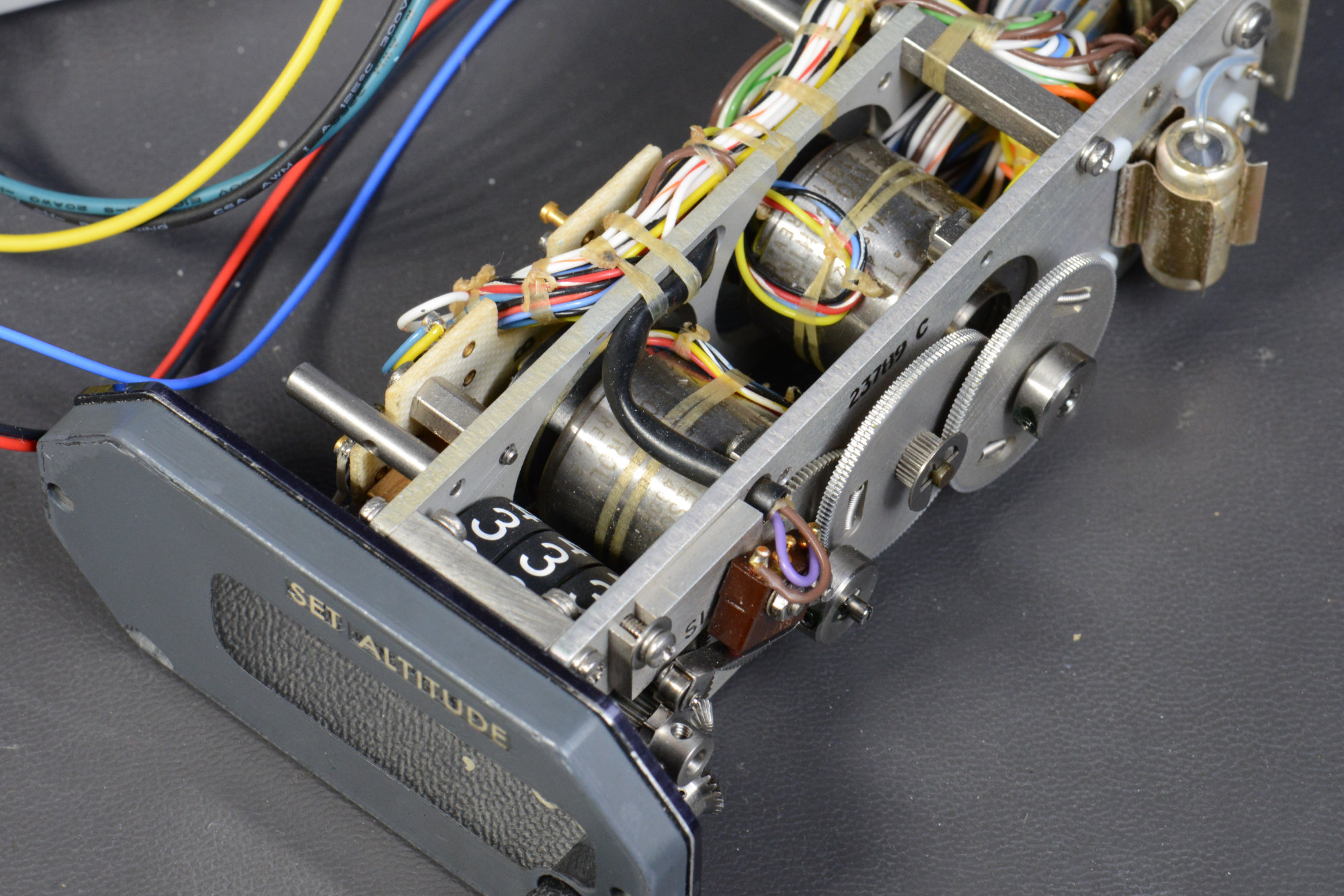
The altitude alerter contains two differential resolvers. The front resolver is the fine altitude resolver. It goes through one complete rotation every 5000 feet. The rear resolver is the coarse altitude resolver. It goes through one complete rotation every 135,000 feet.
I have an old aircraft altitude alerter that contains two synchro resolvers as shown in the photo above. The altitude alerter takes in a pair of synchro format voltages indicating the coarse and fine altitude of the aircraft from the altimeter, computes the difference between the altimeter altitude and the set altitude using a pair of synchro resolvers, and if the difference exceeds a certain distance, sounds a warning to the pilots that they’ve deviated from their set altitude.
Ordinarily, the coarse resolver takes in synchro format voltages and outputs a sine wave whose amplitude is proportional to the difference between the altimeter’s coarse synchro shaft angle and the alerter’s coarse synchro shaft angle. Likewise, the fine resolver takes in synchro format voltages and outputs sine and cosine waves whose amplitudes are proportional to the difference between the altimeter’s fine synchro shaft angle and the alerter’s fine synchro shaft angle.
One property of synchro resolvers is that you can use them as synchro transmitters if you connect them backwards. Instead of feeding a three phase signal into the inputs and getting a single phase or two phase signal from the output, you can feed a single phase signal into the output and get a three phase signal on the input.
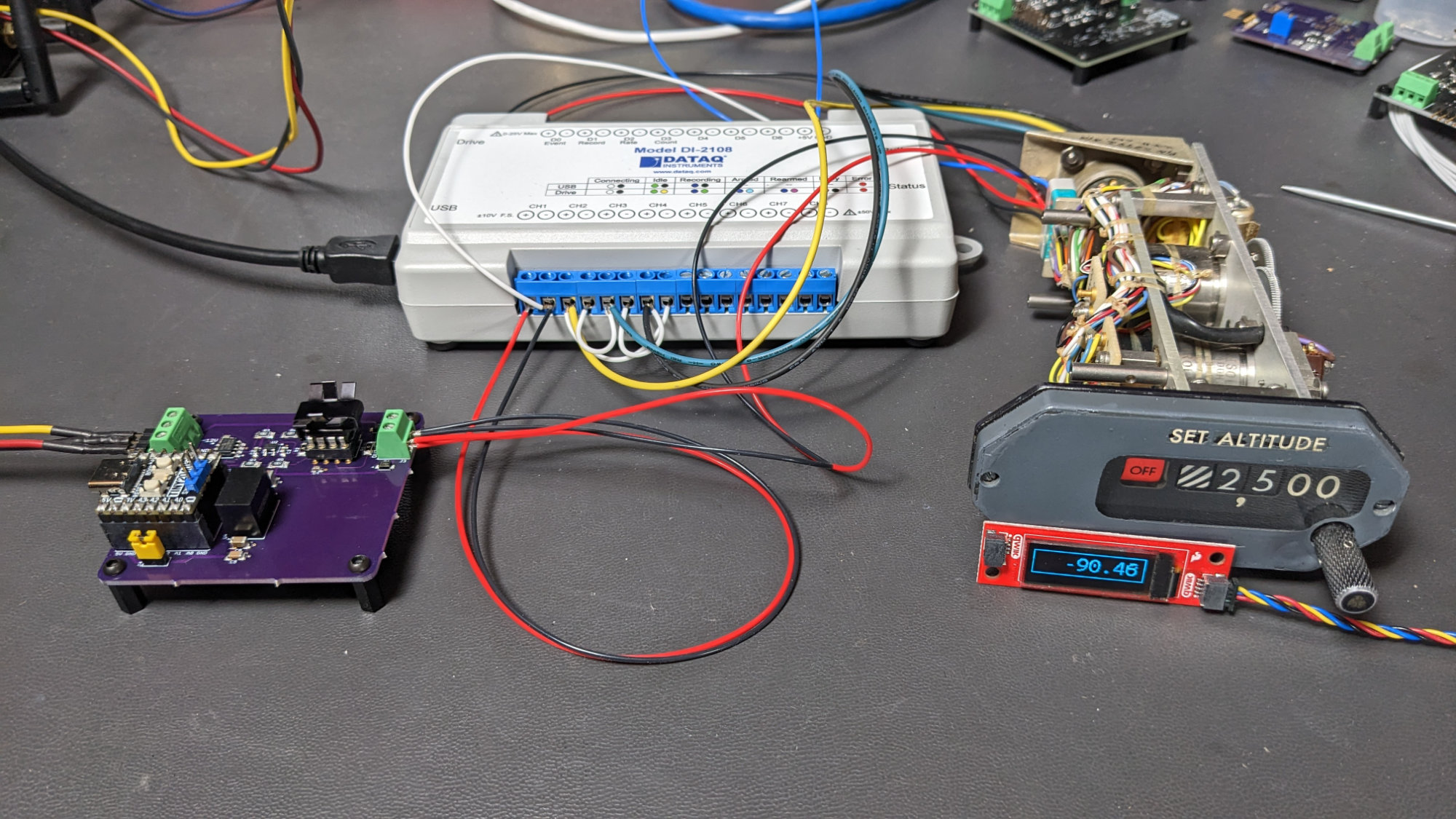
The test setup with the synchro transmitter replaced with the altitude alerter’s fine resolver wired as a synchro transmitter. This permits repeatable adjustment / setting of the synchro shaft angle for testing the tracking converter.
I hooked up the fine resolver’s sine output to my voltage source and grounded the fine resolver’s cosine output. I then connected the resolver’s fine three phase input to the input of the Dataq data acquisition hardware as shown in the photo above.

Here’s a graphic showing the measured angles and altitudes along the unit circle.
With this setup, I had a precise and repeatable way of testing the synchro-to-digital converter. I proceeded to collect some measurements:
- 0 feet: 90°
- 1000 feet: -18°
- 2000 feet: -54°
- 2500 feet: -90°
- 3000 feet: -126°
- 4000 feet: 162°
- 5000 feet: back to 90°
Since the fine resolver makes one complete revolution every 5000 feet, it’s expected that the altitude alerter would loop back to 90° at 5000 feet. I went through the complete range of altitudes from -10,000 feet to +60,00 feet in both directions stopping at various points along the way and the computed output angles were precise and repeatable.
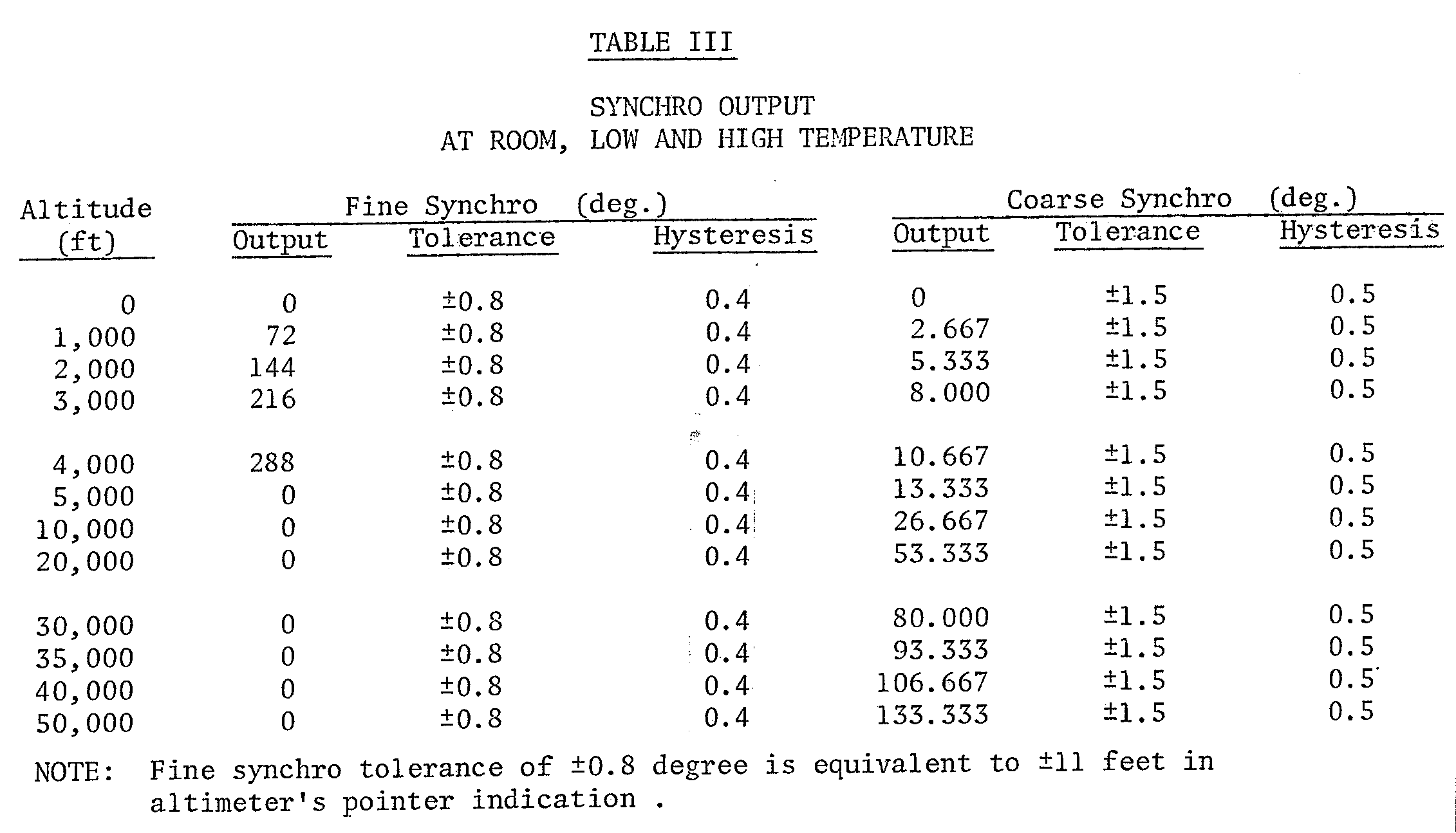
Table III from United Instruments Servoed Encoding Altimeter 5506-S Series datasheet.
It is curious that 0 feet is 90° and not 0°. I could not find any documentation on the altitude alerter that listed a definitive shaft angle for 0 feet. I did find a datasheet on another manufacturer’s encoding altimeter. A table in it (shown above) states 0 feet should be 0°.
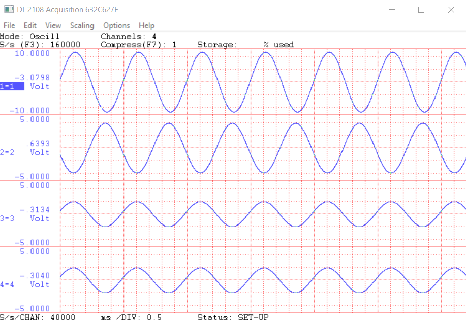
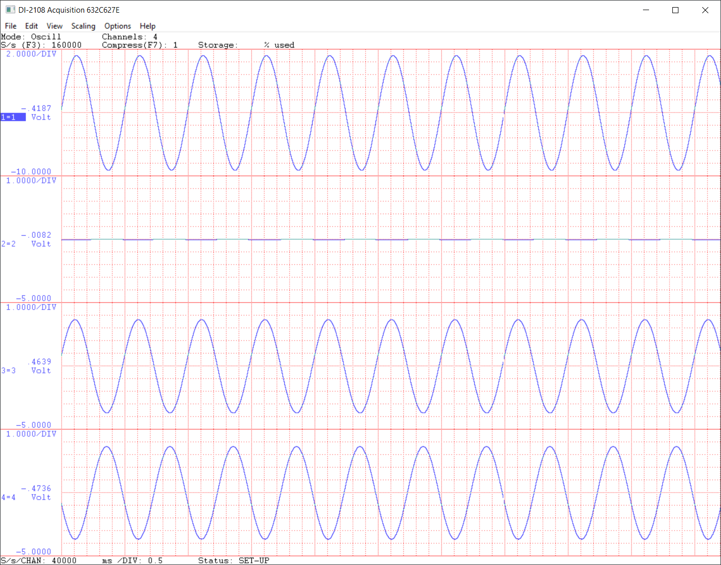
Altitude alerter fine synchro voltages with alerter set to 0 feet. Note that the first trace is Vr1-Vr2 = -(Vr2-Vr1).
Perplexed, I set the alerter for 0 feet, captured the synchro signals, and plotted them above. I then calculated the expected amplitudes of the synchro signals for 90°. The top graph in this case is VR1 – VR2 so a minus sine has to be included in the calculations below. The remaining signals in order are VS1 – VS3, VS3 – VS2, and VS2 – VS1.
>> -sin(90*pi/180)
ans = -1
>> -sin((90+120)*pi/180)
ans = 0.5000
>> -sin((90-120)*pi/180)
ans = 0.5000
According to these calculations, for an angle of 90°, we should see relative amplitudes of -1, 0.5, and 0.5 which we do so the fine synchro is definitely at 90° at 0 feet and there is not an error in my tracking synchro-to-digital converter.
This could just be a difference between different manufacturer’s equipment and 90° is the correct answer. The output can be changed to 0° at 0 feet to match the United Instruments datasheet by subtracting the computed angle from a constant when calculating the error. There’s a comment in the code to this effect. Without schematics of the alerter or datasheets on the resolvers, it’s also possible I have some wires crossed somewhere.
I repeated this experiment with the alerter’s coarse resolver and learned that the coarse resolver shaft turns at 1/27th the rate of the fine resolver shaft. I was able to verify the 1:27 ratio against a data sheet for the alerter.
Demonstration Video
The video above is a quick overview of the test setup and demonstration of the tracking synchro-to-digital converter. In the video, I’m using the version of the Python code that places 0 feet at 0° with the angle increasing as the altitude is increased.
Final Thoughts
In this project, I demonstrated that it was possible to build a tracking synchro-to-digital converter using modern hardware. I went through the basics of synchro transmitters and synchro-to-digital converters. I modeled the converter, built an AC source to power the synchro transmitter, selected off-the-shelf hardware to digitize the output of the synchro transmitter, and implemented a real time synchro-to-digital converter using an embedded x86 system.
Finally, I tested the converter using both a standalone synchro transmitter and, for more precision and repeatability during the testing, a synchro resolver wired as a synchro transmitter in an old aircraft altitude alerter. If I were to continue this project, I’d like to digitize both the coarse and fine synchros on the altitude alerter, convert both to angles, and merge the coarse and fine angles into a single high-precision angle output.
This project has been a very interesting look into the past and at how some aircraft avionics work, but I would stick to potentiometers and encoders for most of my hobby projects because they’re far simpler to interface to a microcontroller than the synchro transmitter and I don’t need the accuracy or resolution afforded by a synchro.
Downloads
The following downloads are available for this project.
- Octave model of the synchro-to-digital converter: model.m
- Python implementation of the synchro-to-digital converter: convert.py
- LTSpice simulation of DAC and opamp: offset-dac-circuit.asc
- Reference voltage source Eagle schematic: ref-gen-board.sch
- Reference voltage source Eagle layout: ref-gen-board.brd
- Raspberry Pi Rp2040 Pico sine wave generator: main.cpp
These files are also available in the github repo for the project.
References
Analog Devices: Synchro and Resolver Conversion Handbook, 1980